data("CASchools", package = "AER")
CASchools$STR = CASchools$students / CASchools$teachers
CASchools$score = (CASchools$read + CASchools$math) / 25 Effects
Section 4 defined marginal effects as changes in the population conditional expectation function (CEF).
We now ask:
- How can a regression relationship be interpreted?
- How do we calculate and interpret effects when the relationship is nonlinear?
5.1 Causality
Recall the fitted wage-education regression from Section 4:
\widehat m(z)=-16.45+2.90z.
Thus,
\widehat m(z+1)-\widehat m(z)=2.90.
Consider two interpretations:
- Estimated association: According to the fitted regression, people with one more year of education earn, on average, USD 2.90 more per hour.
- Causal claim: One additional year of education would increase average hourly wage by USD 2.90.
The fitted regression supports the first statement as an estimated association. The fitted slope 2.90 is the sample estimate of the corresponding population regression slope \beta_2.
When both Y_i and Z_i have finite, positive variances, Equation 4.5 and the definition of correlation imply
\beta_2 =\frac{\mathrm{Cov}(Y_i,Z_i)}{\mathrm{Var}(Z_i)} =\mathrm{Corr}(Y_i,Z_i) \frac{\mathrm{sd}(Y_i)}{\mathrm{sd}(Z_i)}.
Thus, the population regression slope is an association. It is the correlation multiplied by the scale factor \mathrm{sd}(Y_i)/\mathrm{sd}(Z_i). This identity contains no causal statement.
Counterfactual Outcomes
The causal claim asks what would happen to the same people’s wages under a different education level.
For each person, we observe only the wage earned at the actual education level. We do not observe what the same person would have earned at another education level. This unobserved wage is a counterfactual outcome.
Let Y_i(z) denote the wage person i would earn if they had z years of education. The outcomes under different possible education levels are called potential outcomes.
Suppose the person’s actual education is Z_i=z. We then observe
Y_i=Y_i(z),
but we do not observe Y_i(z+1).
The individual causal effect of one additional year of education is
Y_i(z+1)-Y_i(z).
The population average causal effect of a change from z to z+1 years of education is
E[Y_i(z+1)-Y_i(z)] =E[Y_i(z+1)]-E[Y_i(z)]. \tag{5.1}
Here, E[Y_i(z+1)] is the average wage if everyone had z+1 years of education, while E[Y_i(z)] is the average wage if everyone had z years.
Like all population means, these quantities must be estimated from sample data. The additional difficulty is that each person is observed at only one education level.
Random Assignment
An idealized randomized controlled trial (RCT) addresses this difficulty through random assignment.
Suppose people could be randomly assigned to z or z+1 years of education. Each person would still reveal only one potential outcome.
Random assignment would make the two groups comparable on average. Their sample mean wages could therefore estimate the corresponding potential-outcome means.
The difference between the two sample means would estimate the population average causal effect in Equation 5.1. It would not reveal any person’s individual causal effect.
Observational Comparisons
In a survey or another observational study, the researcher observes rather than assigns education.
The population CEF compares people who actually have different education levels:
m(z) =E[Y_i\mid Z_i=z] =E[Y_i(z)\mid Z_i=z].
Hence,
m(z+1)-m(z) = E[Y_i(z+1)\mid Z_i=z+1] - E[Y_i(z)\mid Z_i=z].
The population average causal effect instead compares
E[Y_i(z+1)]-E[Y_i(z)].
The CEF compares two groups of people who actually have different education levels. These groups may differ systematically in relevant pre-existing characteristics. Therefore, the CEF difference need not equal the population average causal effect.
The CEF difference may reflect both:
- Effect of education: Education itself may increase productivity and wages.
- Differences between groups: Pre-existing differences in ability, motivation, family background, resources, or prior academic achievement may affect both education and wages.
Only the first represents the causal effect of education. Because of the second, the observed wages of one education group need not show what the other group would have earned at that education level.
Correlation does not imply causation.

We next examine how such group differences affect the regression coefficient.
5.2 Confounding
Suppose family background affects both education and wage.
We use the following notation:
- Y_i is the outcome: hourly wage.
- D_i is the regressor of interest: education.
- C_i is a possible control: maternal education measured in years.
The regressor of interest is the variable whose change and possible effect on Y_i we want to study.
If C_i is included as another regressor and held fixed in the comparison, it is a control variable.
Maternal education is one aspect of family background. It is a confounder if it affects both the person’s education and wage.
A directed acyclic graph (DAG) summarizes a proposed causal structure. An arrow represents a direct causal effect, not just a correlation.
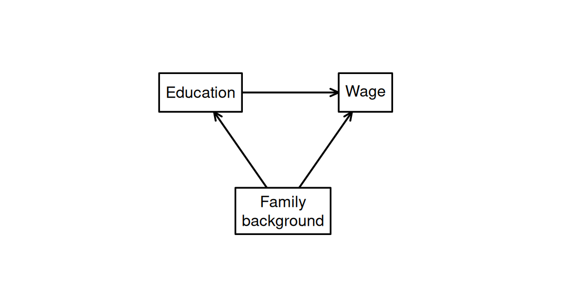
People with more education may also have more highly educated mothers.
If maternal education also affects wage, some of the wage difference may be due to maternal education rather than education itself. A simple regression does not separate these two sources.
In a linear regression, this problem appears as omitted-variable bias.
To see how, consider C_i as the scalar control in the linear population model
Y_i=\beta_1+\beta_DD_i+\gamma C_i+u_i, \qquad E[u_i\mid D_i,C_i]=0, where Y_i, D_i, and C_i have finite second moments and \mathrm{Var}(D_i)>0. As in Section 4, assume no perfect multicollinearity among the regressors.
Here, \beta_D is the population slope for education when maternal education is held fixed.
It describes a conditional association.
As in Section 4.2, the zero conditional mean implies \mathrm{Cov}(D_i,u_i)=0. The covariance rules therefore give \mathrm{Cov}(Y_i,D_i) =\beta_D\mathrm{Var}(D_i) +\gamma\mathrm{Cov}(C_i,D_i).
Dividing by \mathrm{Var}(D_i) gives the population slope from regressing Y_i only on D_i: \widetilde\beta_D =\frac{\mathrm{Cov}(Y_i,D_i)}{\mathrm{Var}(D_i)} =\beta_D +\gamma\frac{\mathrm{Cov}(D_i,C_i)}{\mathrm{Var}(D_i)}. \tag{5.2}
In the wage-education regression above, \widetilde\beta_D is the simple-regression slope previously denoted by \beta_2. The tilde distinguishes it from \beta_D, which holds maternal education fixed.
The second term in Equation 5.2 is the omitted-variable bias in this linear setup.
It is nonzero when both \gamma\neq0 \qquad\text{and}\qquad \mathrm{Cov}(D_i,C_i)\neq0.
In this example, \gamma\neq0 means that wage varies with maternal education when the person’s education is held fixed. The condition \mathrm{Cov}(D_i,C_i)\neq0 means that the person’s education and maternal education vary together.
If maternal education is positively associated with the person’s education and its conditional wage coefficient is positive, the simple-regression slope exceeds the slope holding maternal education fixed.
Confounding is the causal reason for including C_i. Omitted-variable bias describes how leaving it out changes the population regression slope.
Controlling for maternal education means comparing people with different education levels whose mothers have the same number of years of education.
With several controls, we collect them in \boldsymbol C_i and write the population CEF as m(d,\boldsymbol c)=E[Y_i\mid D_i=d,\boldsymbol C_i=\boldsymbol c].
As in Section 4.8, \beta_D is the marginal effect in an additive linear CEF. We compare different values of D_i while holding all controls fixed.
Controls address confounding only when they are chosen appropriately. The next subsection explains why not every control is appropriate.
5.3 Good and Bad Controls
Whether a variable is a good or bad control depends on the research question and the causal effect of interest.
The same variable may therefore be a good control for one question and a bad control for another.
We consider the total effect of education on wage. This includes every pathway through which education may affect wage.
Confounders
Because family background affects both education and wage in Figure 5.1, people with different education levels may have different average wages even if education itself has no effect on wage.
For the total effect, an appropriate set of measured confounders can form a good control set. Holding them fixed can make the education groups more comparable.
Maternal education is one possible control. Other possible measures in micro surveys include paternal education, parents’ occupations during childhood, and childhood household resources.
Maternal education alone need not capture every relevant difference in family background.
Confounding variables are often determined before the regressor.
Mediators
A mediator is caused by the regressor and then affects the outcome.
Education may improve access to higher-paying job positions. Part of its total effect on wage then operates through job position.
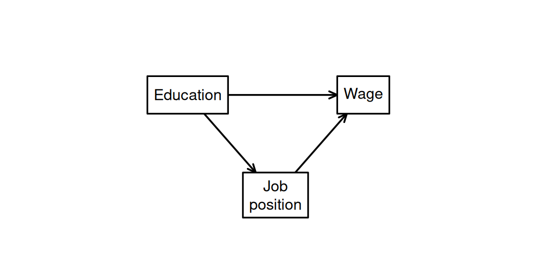
Holding job position fixed compares people with different education but the same position.
In this causal structure, holding job position fixed excludes the pathway through better positions. The resulting comparison does not capture the total effect of education.
Professional sector or later qualifications can also be mediators when education affects them and they in turn affect wage.
Such variables may be relevant when an effect that does not operate through them is the target. That is a different research question.
Colliders
A collider is a variable that is influenced by two other variables.
Suppose, for illustration, that both education and wage increase life satisfaction.
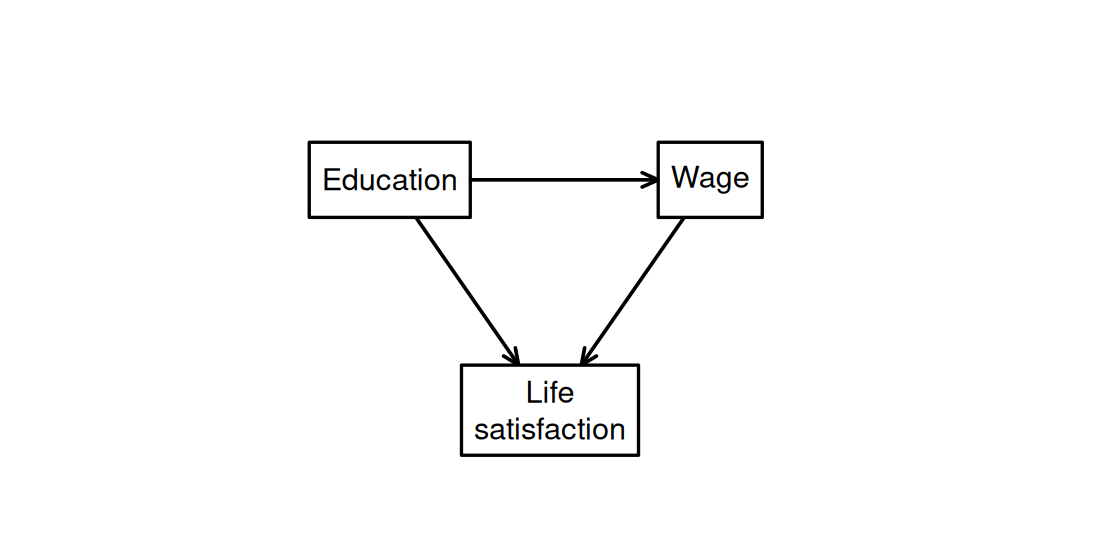
Controlling for life satisfaction means comparing people with the same level of life satisfaction.
A person with more education but a lower wage may then have the same life satisfaction as a person with less education but a higher wage.
Restricting the comparison to equal life satisfaction can therefore introduce a negative association between education and wage—even if education increases wages.
The resulting wage comparison mixes the effect of education with an association created by selecting people with equal life satisfaction. It does not isolate the total causal effect of education on wage.
In this causal structure, life satisfaction is therefore a bad control for the total effect of education on wage.
Choosing Controls
Variables determined before the regressor are often more plausible controls than variables caused by it.
A variable is not a good control just because it predicts the outcome, is correlated with the regressor, improves the fit of the regression, or stabilizes a coefficient.
Control selection requires a causal argument and depends on the effect of interest.
For any chosen controls, m(d,\boldsymbol c) describes a conditional association in the population.
Controlling for all relevant confounders may make this conditional association informative about the total causal effect.
In the causal structures shown above, mediators and colliders are bad controls for the total effect.
Whether these choices are credible depends on knowledge of how the variables are causally related. Regression output alone cannot establish it.
In particular, the condition E[u_i\mid D_i,\boldsymbol C_i]=0 ensures that the linear equation is the CEF for Y_i. It does not show that the controls remove confounding.
Without a credible causal argument, the result remains a conditional association.
5.4 Class Size
We return to the CASchools data introduced in Section 4. They contain 420 California school districts.
The outcome is the district’s average test score. The student-teacher ratio STR is the average number of students per teacher and serves as a measure of class size.
We are interested in the total effect of increasing the student-teacher ratio on test scores.
The variable english is the percentage of English learners, lunch is the percentage eligible for subsidized lunch, and expenditure is expenditure per pupil.
We compare three specifications. Relative to the controlled regression in Section 4, Model (2) adds subsidized-lunch eligibility. Model (3) also includes expenditure per pupil.
Each column in the table is one regression. The rows report coefficient estimates and a blank cell means that the variable is not included.
| (1) | (2) | (3) | |
|---|---|---|---|
| Constant | 698.933 | 700.150 | 665.988 |
| Student-teacher ratio | -2.280 | -0.998 | -0.235 |
| English learners (%) | -0.122 | -0.128 | |
| Subsidized lunch (%) | -0.547 | -0.546 | |
| Expenditure per pupil | 0.004 | ||
| Num.Obs. | 420 | 420 | 420 |
According to the fitted regressions, school districts with one more student per teacher have, on average:
- Model (1): test scores 2.280 points lower.
- Model (2): test scores 0.998 points lower, comparing districts with the same percentages of English learners and students eligible for subsidized lunch.
- Model (3): test scores 0.235 points lower, comparing districts with those same two percentages and the same expenditure per pupil.
The estimates change because districts with different student-teacher ratios also differ in other ways.
The shares of English learners and students eligible for subsidized lunch may capture pre-existing district characteristics.
Expenditure
Funding and expenditure may refer to resources determined at different stages. The following diagrams illustrate two possible causal stories.
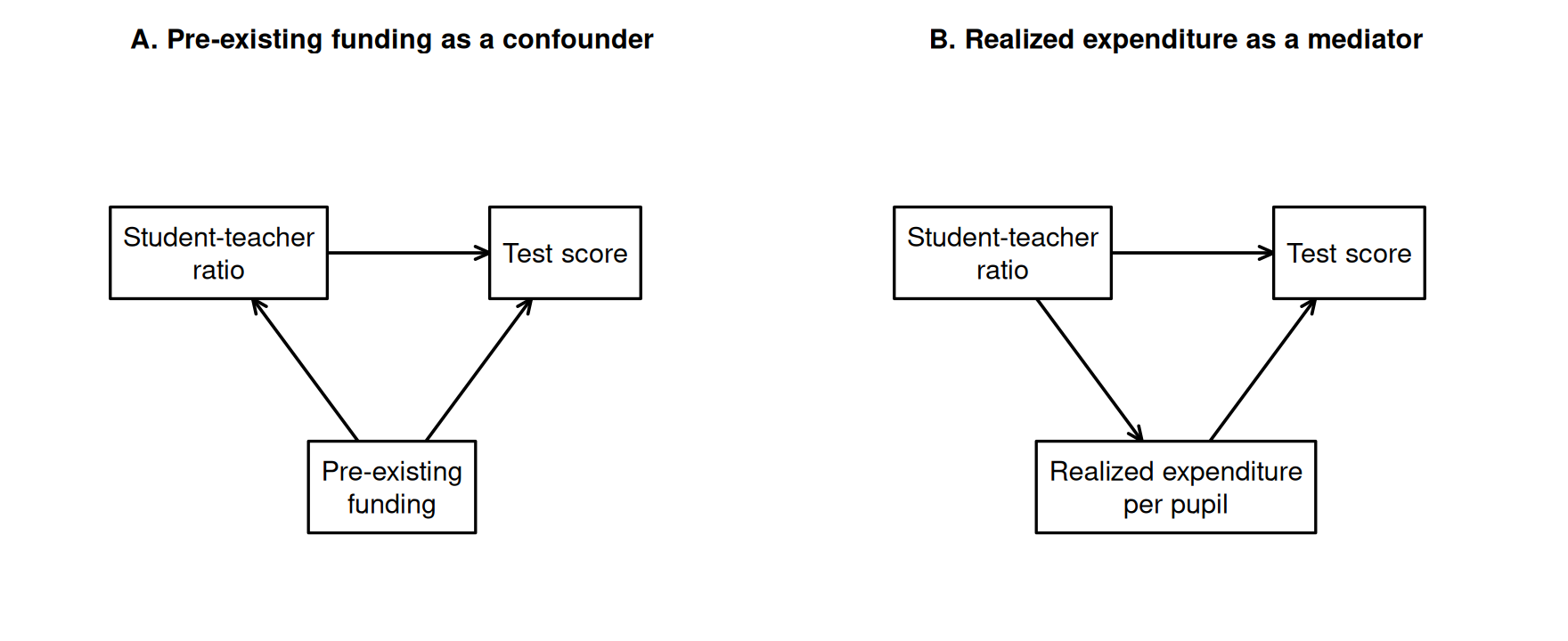
Pre-existing funding may affect both the student-teacher ratio and test scores. It is therefore a possible confounder.
By contrast, realized expenditure per pupil is partly determined by staffing decisions. A policy that hires more teachers lowers the student-teacher ratio but ordinarily raises expenditure per pupil.
Realized expenditure may therefore lie on the causal pathway from such a class-size policy to test scores.
The recorded expenditure measure may reflect both pre-existing resources and spending generated by staffing decisions.
Model (3) compares districts with the same expenditure per pupil but different student-teacher ratios.
For example, lowering the student-teacher ratio while holding expenditure fixed would require lower teacher salaries or lower spending on other school inputs.
Model (3) therefore does not describe the total effect of a class-size policy that also changes expenditure.
Without a justified control strategy, the coefficients remain conditional associations.
5.5 Polynomials
We now examine how the specification determines the size and interpretation of an effect.
Recall from Section 4 the quadratic CEF m_A(a)=\gamma_1+\gamma_2a+\gamma_3a^2.
Its marginal effect is ME_A(a)=\gamma_2+2\gamma_3a.
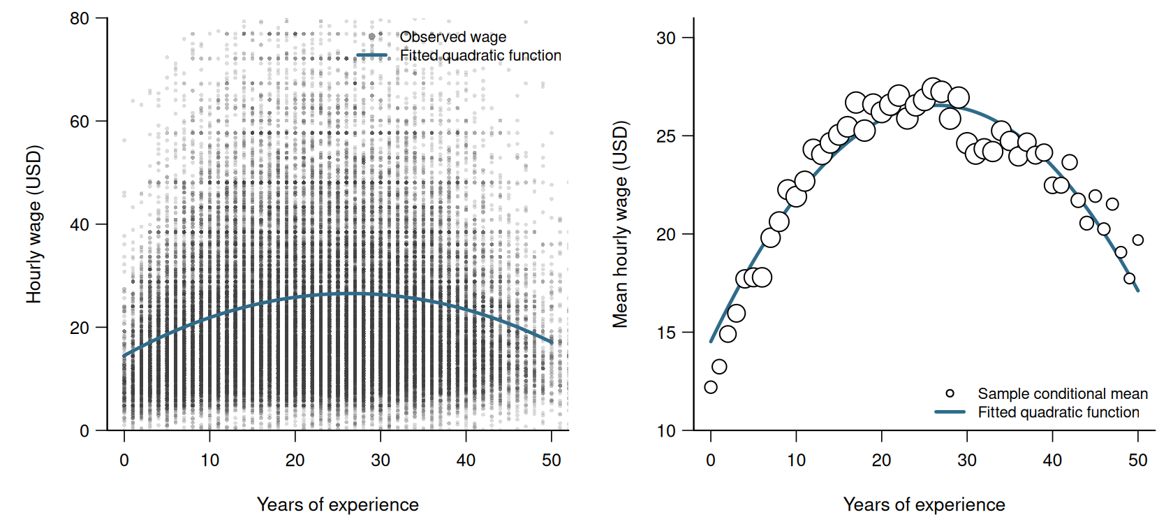
We estimate this specification for wage and experience using OLS, as in Section 4. The regressors are a constant, experience and squared experience.
    (Intercept)      experience I(experience^2)
        14.5198          0.9073         -0.0171
The function I() tells R to include the squared value of experience.
The fitted quadratic function is \widehat m_A(a) =14.520+0.907a-0.0171a^2.
Its estimated marginal effect is \widehat{ME}_A(a) =\widehat\gamma_2+2\widehat\gamma_3a =0.907-2(0.0171)a. \tag{5.3}
At 20 years of experience, \widehat{ME}_A(20) =\widehat\gamma_2+2\widehat\gamma_3\cdot20 =0.223.
The fitted hourly-wage function has a local slope of about USD 0.223 per year of experience at this point.
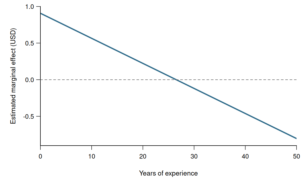
The fitted slope decreases with experience, is zero at about 26.5 years, and is negative thereafter.
5.6 Logarithms
Logarithms are useful when proportional changes are more meaningful than changes in levels.
\log denotes the natural logarithm. This is the standard convention in econometrics.
Since
\frac{\partial \log(x)}{\partial x} = \frac{1}{x},
a small change \Delta x gives
\Delta\log(x) \approx \frac{\Delta x}{x}.
The term \Delta x/x is the proportional change in x. Hence,
100\,\Delta\log(x) \approx \text{percentage change in }x.
Logarithmic Regressor
Suppose X_i>0 and
m_X(x) = E[Y_i\mid X_i=x] = \beta_1+\beta_2\log(x).
This is called a linear-log model.
The marginal effect of X_i is
ME_X(x) = \frac{\partial m_X(x)}{\partial x} = \frac{\beta_2}{x}.
Thus, for a small change \Delta x,
\underbrace{\Delta m_X(x)}_{\substack{\text{absolute change}\\\text{in the conditional mean}}} \approx \beta_2 \underbrace{\frac{\Delta x}{x}}_{\substack{\text{relative change}\\\text{in }X}}.
A one-percent increase in X_i has \Delta x/x=0.01.
Therefore,
A 1% higher value of X_i is associated with a value of Y_i that is approximately \beta_2/100 units higher, on average.
Income and Test Scores
Consider district income and test scores in the CASchools sample. Income is measured in thousands of USD.
(Intercept) log(income)
     557.83       36.42
The fitted linear-log function is \widehat{\text{score}} =557.83+36.42\log(\text{income}).
According to the fitted regression, school districts with 1% higher average income have, on average, test scores about 36.42/100=0.36 points higher.
For comparison, we also estimate a quadratic specification:
(Intercept)      income I(income^2)
  607.30174     3.85099    -0.04231
The fitted quadratic function is \widehat{\text{score}} =607.30+3.851\,\text{income}-0.04231\,\text{income}^2.
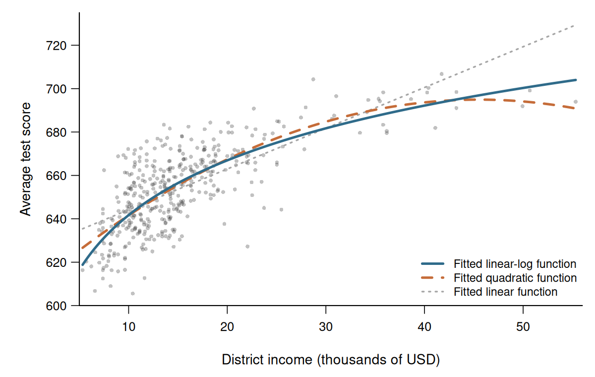
The quadratic and linear-log specifications describe similar relationships over much of the income range.
At higher incomes, the quadratic fit turns downward, while the linear-log fit continues to increase. The estimated marginal effects therefore depend on the chosen specification.
Logarithmic Outcome
We now model the conditional mean of \log(Y_i).
Exponentiating this conditional mean gives the conditional geometric mean of Y_i.
For Y_i>0, define
g_X(x) := \exp\!\left(E[\log(Y_i)\mid X_i=x]\right).
The function g_X(x) is the conditional geometric mean of Y_i.
The geometric mean is another measure of the center of a positive variable. It is always less than or equal to the usual arithmetic mean: g_X(x)\leq E[Y_i\mid X_i=x].
Consider the log-linear model
E[\log(Y_i)\mid X_i=x] = \beta_1+\beta_2x.
It implies
g_X(x) = \exp(\beta_1+\beta_2x).
Thus, g_X(x) is convex. It is increasing when \beta_2>0 and decreasing when \beta_2<0.
Its derivative is
\frac{\partial g_X(x)}{\partial x} = \beta_2g_X(x).
Therefore, for a small change \Delta x,
\underbrace{\frac{\Delta g_X(x)}{g_X(x)}}_{\substack{\text{relative change in the}\\\text{conditional geometric mean}}} \approx \beta_2 \underbrace{\Delta x}_{\substack{\text{absolute change}\\\text{in }X}}.
For a one-unit change, this approximation is accurate when |\beta_2| is small:
A one-unit higher value of X_i is associated with an approximately 100\beta_2 percent higher value of Y_i, on average.
Here, “on average” refers to the conditional geometric mean, not the arithmetic mean. This distinction is often omitted in applied econometrics, and we use that shorthand for models with a logged outcome.
The coefficient \beta_2 is the semielasticity of the conditional geometric mean.
Wage and Education
(Intercept)   education
      1.440       0.108
Here, e denotes years of education.
The corresponding fitted conditional geometric mean is \widehat g_E(e) =\exp(1.440+0.108e).
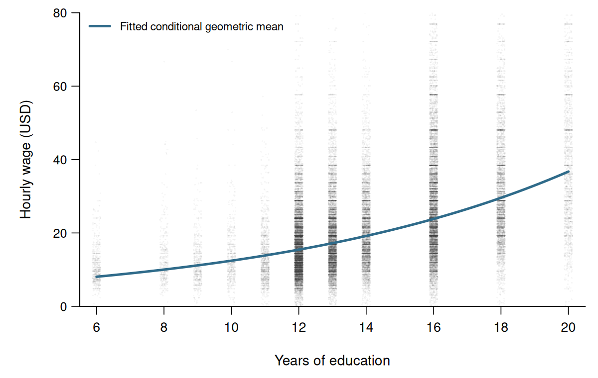
The fitted conditional geometric mean is convex.
According to the fitted regression, people with one more year of education have, on average, hourly wages approximately 100\cdot0.108=10.8 percent higher.
Both Variables
When both variables are logged,
E[\log(Y_i)\mid X_i=x] = \beta_1+\beta_2\log(x).
This is called a log-log model.
It implies
g_X(x) = \exp(\beta_1)x^{\beta_2}.
Its derivative is
\frac{\partial g_X(x)}{\partial x} = \beta_2\exp(\beta_1)x^{\beta_2-1} = \beta_2\frac{g_X(x)}{x}.
Therefore, for a small change \Delta x,
\underbrace{\frac{\Delta g_X(x)}{g_X(x)}}_{\substack{\text{relative change in the}\\\text{conditional geometric mean}}} \approx \beta_2 \underbrace{\frac{\Delta x}{x}}_{\substack{\text{relative change}\\\text{in }X}}.
Thus, \beta_2 is the elasticity of the conditional geometric mean:
A 1% higher value of X_i is associated with an approximately \beta_2 percent higher value of Y_i, on average.
Summary
| Model | Comparison in X_i | Approximate difference | Population quantity |
|---|---|---|---|
| Linear-log | 1% higher | \beta_2/100 units | Conditional mean of Y_i |
| Log-linear | One unit higher | 100\beta_2 percent | Conditional geometric mean of Y_i |
| Log-log | 1% higher | \beta_2 percent | Conditional geometric mean of Y_i |
Other included regressors are held fixed.
All three interpretations use small-change approximations. They work best when the percentage changes in the variables that are logged are small.
5.7 Interactions
An interaction allows the effect of one regressor to depend on another.
Let F_i be the female dummy variable (i.e., F_i=1 for women). Consider m(e,f) =\beta_1+\beta_2e+\beta_3f+\beta_4ef.
For men (F_i=0), m(e,0)=\beta_1+\beta_2e.
For women (F_i=1), m(e,1)=(\beta_1+\beta_3)+(\beta_2+\beta_4)e.
Comparing women with men:
- \beta_3 is the difference in intercepts.
- \beta_4 is the difference in education slopes.
For wage, education, and female, we estimate
     (Intercept)        education           female education:female
         -19.373            3.341            6.394           -0.997
In the formula, education * female includes education, female, and their product.
The fitted function is \begin{aligned} \widehat m(e,f) &=\widehat\beta_1+\widehat\beta_2e +\widehat\beta_3f+\widehat\beta_4ef \\ &=-19.373+3.341e+6.394f-0.997ef. \end{aligned}
The estimated marginal effect of education is \frac{\partial\widehat m(e,f)}{\partial e} =\widehat\beta_2+\widehat\beta_4f =3.341-0.997f.
The estimated marginal effect is USD 3.34 per additional year of education for men and USD 2.34 for women.
The interaction coefficient \widehat\beta_4=-0.997 means that the fitted education slope is USD 1.00 lower for women than for men.
Because the fitted function is linear in education within each group, these slopes also describe the fitted one-year differences. According to the fitted regression:
- Among men, those with one more year of education earn, on average, USD 3.34 more per hour.
- Among women, those with one more year of education earn, on average, USD 2.34 more per hour.
The fitted mean hourly-wage difference between women and men with the same education level e is \widehat m(e,1)-\widehat m(e,0) =\widehat\beta_3+\widehat\beta_4e =6.394-0.997e.
At 12 years of education, \widehat m(12,1)-\widehat m(12,0) =6.394-0.997\cdot12 =-5.57.
According to the fitted regression, women with 12 years of education earn, on average, USD 5.57 less per hour than men with the same education level.
Thus, neither the coefficient on female nor the interaction coefficient alone is the group difference at every education level.
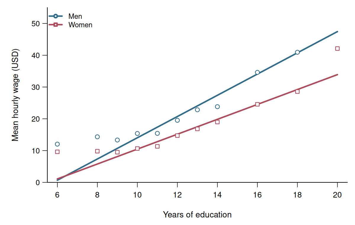
The education slopes are conditional associations within each group.
A causal interpretation of the education effect would require a credible argument that the comparison is not confounded. The group difference itself is descriptive.
The next section develops statistical inference for estimated regression coefficients and effects.