cps = read.csv("cps.csv")
n = length(cps$region)  #sample size
pmf = table(cps$region)/n #relative frequencies
pmf
        1         2         3         4
0.1911434 0.2369832 0.3169761 0.2548973 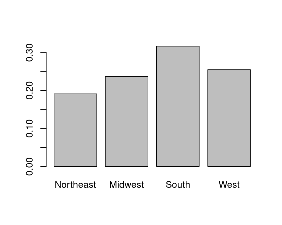
An event is a collection of different outcomes, typically in form of open, half-open, or closed intervals, or unions of multiple intervals.
The probability distribution F_Y assigns probabilities to all possible events of Y. The cumulative distribution function (CDF) fully characterizes the probability distribution:
Cumulative Distribution Function (CDF)
The CDF of a random variable Y is F_Y(a) := P(Y \leq a), \quad a \in \mathbb R.
Any nondecreasing right-continuous function F_Y(a) with \lim_{a \to -\infty} F_Y(a) = 0 and \lim_{a \to +\infty} F_Y(a) = 1 defines a valid CDF.
For a more detailed introduction to probability theory, see my tutorial at probability.svenotto.com.
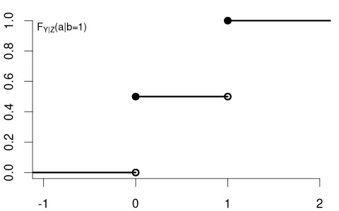
Consider the coin toss binary random variable Y = \begin{cases} 1 & \text{if outcome is heads,} \\ 0 & \text{if outcome is tails.} \end{cases} The CDF for a fair coin is F_Y(a) = \begin{cases} 0 & a < 0, \\ 0.5 & 0 \leq a < 1, \\ 1 & a \geq 1, \end{cases}
with the following CDF plot:
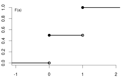
A random variable with a CDF that has jumps and is flat between these jumps is called a discrete random variable.
Let F_Y(a^-) = \lim_{\varepsilon \to 0, \varepsilon > 0} F_Y(a-\varepsilon) denote the left limit of F_Y at a.
That means, for the coin toss, we have point values F_Y(0) = 0.5 and F_Y(1) = 1 and the left-hand limits F_Y(0^-) = 0 and F_Y(1^-) = 0.5.
The point probability P(Y = a) represents the size of the jump at a in the CDF F_Y(a): P(Y=a) = F_Y(a) - F_Y(a^-). Because CDFs are right-continuous, jumps can only be seen when approaching a point a from the left.
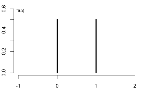
Probability Mass Function (PMF)
The probability mass function (PMF) of a discrete random variable Y is \pi_Y(a) := P(Y = a) = F_Y(a) - F_Y(a^-), \quad a \in \mathbb R.
The PMF of the coin variable is \pi_Y(a) = P(Y=a) = \begin{cases} 0.5 & \text{if} \ a \in\{0,1\}, \\ 0 & \text{otherwise}. \end{cases}
Suppose you conduct a survey where you ask a randomly selected person about their years of education, with the following answer options: Y \in \{10, 12, 14, 16, 18, 21\}.
The education variable is a discrete random variable. It may have the following CDF and PMF:
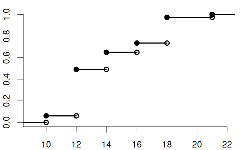
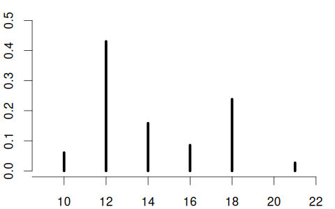
Here, the PMF is \pi_Y(a) = \begin{cases} 0.06 & \text{if } a = 10 \\ 0.43 & \text{if } a = 12 \\ 0.16 & \text{if } a = 14 \\ 0.08 & \text{if } a = 16 \\ 0.24 & \text{if } a = 18 \\ 0.03 & \text{if } a = 21 \\ 0 & \text{otherwise} \end{cases}
The support \mathcal Y is the set of all values that Y can take with non-zero probability: \mathcal{Y} = \{ a \in \mathbb{R} : \pi_Y(a) > 0 \}.
For the coin variable, the support is \mathcal{Y} = \{0, 1\}, while for the education variable, the support is \mathcal{Y} = \{10, 12, 14, 16, 18, 21\}.
The sum of \pi_Y(a) over the support is 1: \sum_{a\in\mathcal Y}\pi_Y(a)=1.
For the tail probabilities we have the following rules:
For intervals (with a < b):
For a continuous random variable Y, the CDF F_Y(a) has no jumps and is continuous. The left limits F_Y(a^-) equal the point values F_Y(a) for all a, which means that the point probabilities are zero: P(Y=a) = F_Y(a) - F_Y(a^-) = 0.
Probability is distributed continuously over intervals. Unlike discrete random variables, which are characterized by both the PMF and the CDF, continuous variables have \pi_Y(a)=P(Y=a)=0 for every point, so the PMF is not a useful concept here.
Instead, they are described by the probability density function (PDF), which serves as the continuous analogue of the PMF. If the CDF is differentiable, the PDF is given by its derivative:
Probability Density Function (PDF)
The probability density function (PDF) or simply density function of a continuous random variable Y is the derivative of its CDF: f_Y(a) = \frac{d}{da} F_Y(a).
Conversely, the CDF can be obtained from the PDF by integration: F_Y(a) = \int_{-\infty}^a f_Y(u) \, du
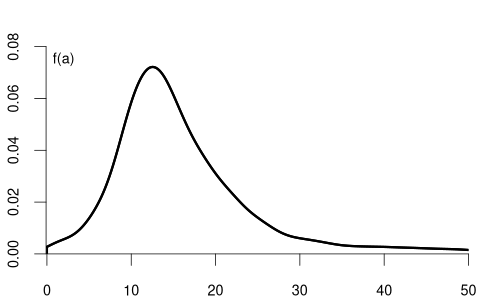
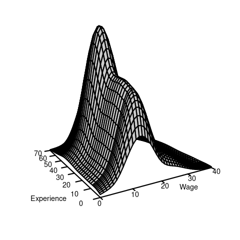
If you ask a random person about their income per working hour in EUR, there are infinitely many potential answers. Any (non-negative) real number may be an outcome. The set of possible results of such a random variable is a continuum of different wage levels.
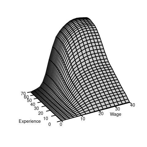
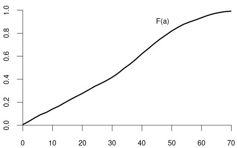
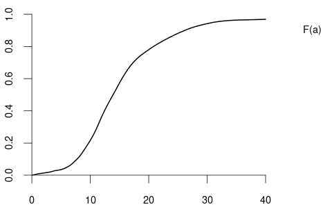
The CDF and PDF of wage may have the following form:
Basic Rules for Continuous Random Variables (with a \leq b):
Unlike the PMF, which directly gives probabilities, the PDF does not represent probability directly. Instead, the probability is given by the area under the PDF curve over an interval.
It is important to note that for continuous random variables, the probability of any single point is zero. This is why, as shown in the last rule above, the inequalities (strict or non-strict) don’t affect the probability calculations for intervals. This stands in contrast to discrete random variables, where the inclusion of endpoints can change the probability value.
The distribution of wage may differ between men and women. Similarly, the distribution of education may vary between married and unmarried individuals. In contrast, the distribution of a coin flip should remain the same regardless of whether the person tossing the coin earns 15 or 20 EUR per hour.
The conditional cumulative distribution function (conditional CDF), F_{Y|Z=b}(a) = F_{Y|Z}(a|b) = P(Y\leq a|Z=b), represents the distribution of a random variable Y given that another random variable Z takes a specific value b. It answers the question: “If we know that Z=b, what is the distribution of Y?”
For example, suppose that Y represents wage and Z represents education:
Since wage is a continuous variable, its conditional distribution given any specific value of another variable is usually also continuous. The conditional density of Y given Z=b is defined as the derivative of the conditional CDF: f_{Y|Z=b}(a) = f_{Y|Z}(a|b) = \frac{d}{d a} F_{Y|Z=b}(a).
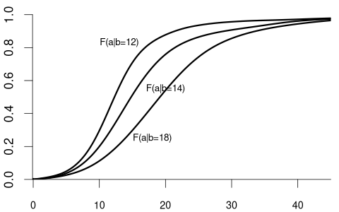
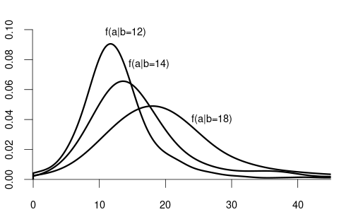
We observe that the distribution of wage varies across different levels of education. For example, individuals with fewer years of education are more likely to earn less than 20 EUR per hour: P(Y\leq 20 | Z=12) = F_{Y|Z=12}(20) > F_{Y|Z=18}(20) = P(Y\leq 20|Z = 18). Because the conditional distribution of Y given Z=b depends on the value b of Z, we say that the random variables Y and Z are dependent random variables.
Note that the conditional CDF F_{Y|Z=b}(a) can only be defined for values of b in the support of Z.
We can also condition on more than one variable. Let Z_1 represent the labor market experience in years and Z_2 be the female dummy variable. The conditional CDF of Y given Z_1 = b and Z_2 = c is: F_{Y|Z_1=b,Z_2=c}(a) = F_{Y|Z_1,Z_2}(a|b,c) = P(Y \leq a|Z_1=b, Z_2=c).
For example:
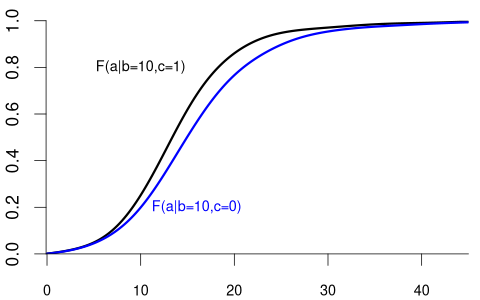
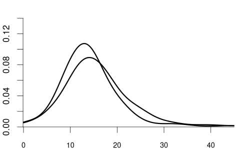
Clearly, the random variable Y and the random vector (Z_1, Z_2) are dependent.
More generally, we can condition on the event that a k-variate random vector \boldsymbol Z = (Z_1, \ldots, Z_k)' takes the value \{\boldsymbol Z = \boldsymbol b\}, i.e., \{Z_1 = b_1, \ldots, Z_k = b_k\}. The conditional CDF of Y given \{\boldsymbol Z = \boldsymbol b\} is F_{Y|\boldsymbol Z = \boldsymbol b}(a) = F_{Y|Z_1 = b_1, \ldots, Z_k = b_k}(a).
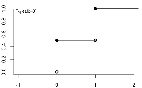
The variable of interest, Y, can also be discrete. Then, any conditional CDF of Y is also discrete. Below is the conditional CDF of education given the married dummy variable:
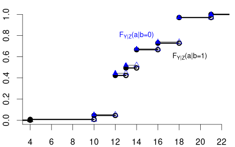
The conditional PMFs \pi_{Y|Z=0}(a) = P(Y = a | Z=0) and \pi_{Y|Z=1}(a)= P(Y = a | Z=1) indicate the jump heights of F_{Y|Z=0}(a) and F_{Y|Z=1}(a) at a.
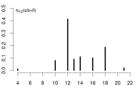
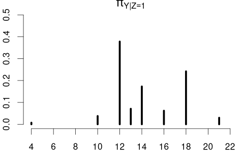
Clearly, education and married are dependent random variables. For example, \pi_{Y|Z=0}(12) > \pi_{Y|Z=1}(12) and \pi_{Y|Z=0}(18) < \pi_{Y|Z=1}(18).
In contrast, consider Y= coin flip and Z= married dummy variable. The CDF of a coin flip should be the same for married or unmarried individuals:
Because F_Y(a) = F_{Y|Z=0}(a) = F_{Y|Z=1}(a) \quad \text{for all} \ a we say that Y and Z are independent random variables.
When we have two random variables Y and Z, we need to understand three related concepts:
The joint CDF describes the probability that both variables simultaneously fall below specified values: F_{Y,Z}(a,b) = P(Y \leq a, Z \leq b).
The marginal CDFs are obtained by “sending the other coordinate to + \infty”: \begin{align*} F_Y(a) &= \lim_{b \to \infty} F_{Y,Z}(a,b) = P(Y \leq a), \\ F_Z(b) &= \lim_{a \to \infty} F_{Y,Z}(a,b) = P(Z \leq b). \end{align*}
When both variables are continuous, the joint PDF is f_{Y,Z}(a,b) = \frac{\partial^2}{\partial a \, \partial b} F_{Y,Z}(a,b) and the marginal PDFs are f_Y(a) = \int_{-\infty}^\infty f_{Y,Z}(a,v) \, dv, \quad f_Z(b) = \int_{-\infty}^\infty f_{Y,Z}(u,b) \, du.
When both variables are discrete, the joint PMF is \pi_{Y,Z}(a,b) = P(Y=a, Z=b), and the marginal PMFs are \pi_Y(a) = \sum_{v \in \mathcal Z} \pi_{Y,Z}(a,v), \quad \pi_Z(b) = \sum_{u \in \mathcal Y} \pi_{Y,Z}(u,b), where \mathcal Y and \mathcal Z are the supports of Y and Z.
If Z is continuous (with f_Z(b) > 0): F_{Y|Z=b}(a) = \int_{-\infty}^a f_{Y|Z=b}(u) \,du = \frac{\frac{\partial}{\partial b} F_{Y,Z}(a,b)}{f_Z(b)}. If Z is discrete (with b \in \mathcal Z): F_{Y|Z=b}(a) = \sum_{u \in \mathcal Y, u \leq a} \pi_{Y|Z=b}(u) = \frac{F_{Y,Z}(a,b) - F_{Y,Z}(a,b^-)}{F_Z(b) - F_Z(b^-)}.
In general or mixed cases, the conditional CDF can be defined through limits: F_{Y|Z=b}(a) = \lim_{\epsilon \to 0, \epsilon > 0} \frac{F_{Y,Z}(a,b + \epsilon) - F_{Y,Z}(a,b - \epsilon)}{F_Z(b + \epsilon) - F_Z(b - \epsilon)}.
At the CDF level (Riemann-Stieltjes form), the joint can be built from a conditional and the other variable’s marginal: F_{Y,Z}(a,b) = \int_{- \infty}^b F_{Y|Z=v}(a) \, d F_Z(v) = \int_{-\infty}^a F_{Z|Y=u}(b) \, dF_Y(u). Special cases:
For PDF/PMF, the product rules are: \begin{align*} f_{Y,Z}(a,b) &= f_{Z|Y=a}(b) f_Y(a) = f_{Y|Z=b}(a) f_Z(b), \\ \pi_{Y,Z}(a,b) &= \pi_{Z|Y=a}(b) \pi_Y(a) = \pi_{Y|Z=b}(a) \pi_Z(b). \end{align*}
In the previous section, we saw that the distribution of a coin flip remains the same regardless of a person’s marital status, illustrating the concept of independence. Let’s now formalize this important concept.
Independence
Y and Z are independent if and only if F_{Y|Z=b}(a) = F_{Y}(a) \quad \text{for all} \ a \ \text{and} \ b.
Note that if F_{Y|Z=b}(a) = F_{Y}(a) for all b, then automatically F_{Z|Y=a}(b) = F_{Z}(b) for all a. Due to this symmetry we can equivalently define independence through the property F_{Z|Y=a}(b) = F_{Z}(b).
Technical Note: Mathematically, the condition is required to hold only for almost every b. That is, for all b except on a set with probability zero under Z. Intuitively, it only needs to hold on the values that Z can actually take. For example, if Z is wage and wages can’t be negative, the condition need not hold for negative b.
The definition naturally generalizes to Z_1, Z_2, Z_3 in a sequential chain form. They are mutually independent if
for all a and for (almost) all (b_1, b_2).
Mutual Independence
The random variables Z_1, \ldots, Z_n are mutually independent if and only if, for each i = 2,\dots,n, F_{Z_i | Z_1=b_1,\ldots,Z_{i-1}=b_{i-1}}(a) = F_{Z_i}(a) for all a and (almost) all (b_1, \ldots, b_{i-1}).
An equivalent viewpoint uses the joint CDF of the vector \boldsymbol Z = (Z_1, \ldots, Z_n)': F_{\boldsymbol Z}(\boldsymbol a) = F_{Z_1, \ldots, Z_n}(a_1, \ldots, a_n) = P(Z_1 \leq a_1, \ldots, Z_n \leq a_n). Then, Z_1, \ldots, Z_n are mutually independent if and only if F_{\boldsymbol Z}(\boldsymbol a) = F_{Z_1}(a_1) \cdots F_{Z_n}(a_n) \quad \text{for all} \ a_1, \ldots, a_n.
An important concept in statistics is that of an independent and identically distributed (i.i.d.) sample. This arises naturally when we consider multiple random variables that share the same distribution and do not influence each other.
i.i.d. Sample / Random Sample
A collection of random variables Y_1, \dots, Y_n is i.i.d. (independent and identically distributed) if:
They are mutually independent: for each i = 2,\dots,n, F_{Y_i | Y_1=b_1, \ldots, Y_{i-1}=b_{i-1}}(a) = F_{Y_i}(a) for all a and (almost) all (b_1, \ldots, b_{i-1}).
They have the same distribution function: F_{Y_i}(a) = F(a) for all i=1,\ldots,n and all a.
For example, consider n coin flips, where each Y_i represents the outcome of the i-th flip (with Y_i=1 for heads and Y_i=0 for tails). If the coin is fair and the flips are performed independently, then Y_1, \ldots, Y_n form an i.i.d. sample with
F(a) = F_{Y_i}(a) = \begin{cases} 0 & a < 0 \\ 0.5 & 0 \leq a < 1 \\ 1 & a \geq 1 \end{cases} \qquad \text{for all} \ i=1, \ldots, n.
Similarly, if we randomly select n individuals from a large population and measure their wages, the resulting measurements Y_1, \ldots, Y_n can be treated as an i.i.d. sample. Each Y_i follows the same distribution (the wage distribution in the population), and knowledge of one person’s wage doesn’t affect the distribution of another’s. The function F is called the population distribution or the data-generating process (DGP).
Often in practice, we work with multiple variables recorded for different individuals or time points. For example, consider two random vectors: \boldsymbol{X}_1 = (X_{11}, \ldots, X_{1k})', \quad \boldsymbol{X}_2 = (X_{21}, \ldots, X_{2k})'.
The conditional distribution function of \boldsymbol{X}_1 given that \boldsymbol{X}_2 takes the value \boldsymbol{b}=(b_1,\ldots,b_k)' is F_{\boldsymbol{X}_1 | \boldsymbol{X}_2 = \boldsymbol{b}}(\boldsymbol{a}) = P(\boldsymbol{X}_1 \le \boldsymbol{a}|\boldsymbol{X}_2 = \boldsymbol{b}), where the vector inequality \boldsymbol{X}_1 \le \boldsymbol{a} means the componentwise inequalities X_{1j} \le a_j for all j =1, \ldots, k hold.
For instance, if \boldsymbol{X}_1 and \boldsymbol{X}_2 represent the survey answers of two different, randomly chosen people, then F_{\boldsymbol{X}_2 | \boldsymbol{X}_1=\boldsymbol{b}}(\boldsymbol{a}) describes the distribution of the second person’s answers, given that the first person’s answers are \boldsymbol{b}.
If the two people are truly randomly selected and unrelated to one another, we would not expect \boldsymbol{X}_2 to depend on whether \boldsymbol{X}_1 equals \boldsymbol{b} or some other value \boldsymbol{c}. In other words, knowing \boldsymbol X_1 provides no information that changes the distribution of \boldsymbol X_2.
Independence of Random Vectors
Two random vectors \boldsymbol{X}_1 and \boldsymbol{X}_2 are independent if and only if F_{\boldsymbol{X}_1 | \boldsymbol{X}_2 = \boldsymbol{b}}(\boldsymbol{a}) = F_{\boldsymbol{X}_1}(\boldsymbol{a}) \quad \text{for all } \boldsymbol{a} \ \text{and (almost) all } \ \boldsymbol{b}.
This definition extends naturally to mutual independence of n random vectors \boldsymbol{X}_1,\dots,\boldsymbol{X}_n, where \boldsymbol{X}_i = (X_{i1},\dots,X_{ik})'. They are called mutually independent if, for each i = 2,\dots,n, F_{\boldsymbol X_i| \boldsymbol X_1=\boldsymbol b_1, \ldots, \boldsymbol X_{i-1}=\boldsymbol b_{i-1}}(\boldsymbol a) = F_{\boldsymbol X_i}(\boldsymbol a) for all \boldsymbol{a} and (almost) all (\boldsymbol{b}_1,\dots,\boldsymbol{b}_{i-1}).
Hence, in an independent sample, what the i-th randomly chosen person answers does not depend on anyone else’s answers.
i.i.d. Sample of Random Vectors
The concept of i.i.d. samples naturally extends to random vectors. A collection of random vectors \boldsymbol{X}_1, \dots, \boldsymbol{X}_n is i.i.d. if they are mutually independent and have the same distribution function F. Formally, F_{\boldsymbol X_i| \boldsymbol X_1=\boldsymbol b_1, \ldots, \boldsymbol X_{i-1}=\boldsymbol b_{i-1}}(\boldsymbol a) = F(\boldsymbol a) for all i=1, \ldots, n, for all \boldsymbol{a}, and (almost) all (\boldsymbol{b}_1,\dots,\boldsymbol{b}_{i-1}).
An i.i.d. dataset (or random sample) is one where each multivariate observation not only comes from the same population distribution F but is independent of the others.
With i.i.d. data Y_1, \ldots, Y_n from a discrete random variable Y with support \mathcal Y, the PMF \pi_Y(a) can be estimated by the empirical PMF \hat \pi_Y(a) = \frac{n(a)}{n}, \quad a \in \mathcal Y where n(a) is the count of observations equal to a.
Let’s load the CPS data from Section 1 and estimate the PMF for region (1 = Northeast, 2 = Midwest, 3 = South, 4 = West):
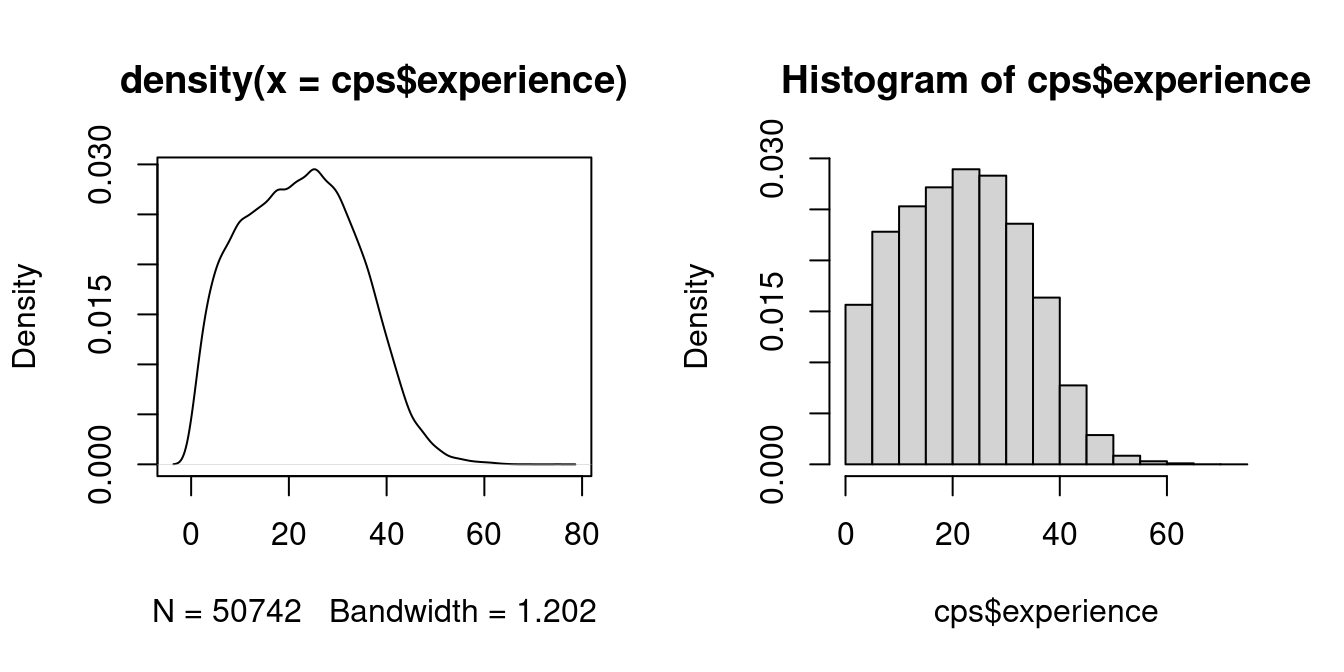
For continuous data, a histogram provides an intuitive estimate of the PDF.
A histogram divides the data range into B bins, each of equal width h, and counts the number of observations n_j within each bin.
The histogram density estimator is \widehat f_Y(a) = \frac{n_j}{nh} \quad \text{for} \ a \ \text{in bin} \ j, so the total area of the rectangles sums to 1.
Suppose we want to estimate the experience density at a = 21 and consider the histogram density estimate with h=5. It is based on the frequency of observations in the interval [20, 25) which is a skewed window about a = 21.
It seems more sensible to center the window at 21, for example [18.5, 23.5) instead of [20, 25). It also seems sensible to give more weight to observations close to 21 and less to those at the edge of the window.
This idea leads to the kernel density estimator of f_Y(a), which is a smooth version of the histogram:
\widehat f_Y(a) = \frac{1}{nh} \sum_{i=1}^n K\Big(\frac{a - Y_i}{h} \Big). Here, K(u) represents a weighting function known as a kernel function, and h > 0 is the bandwidth. A common choice for K(u) is the Gaussian kernel: K(u) = \phi(u) = \frac{1}{\sqrt{2 \pi}} \exp(-u^2/2).
The hist() and density() functions in R automatically choose default values for the number of bins B and the bandwidth h.