library(TeachData)
par(mfrow = c(1,2))
plot(gdp, main = "Nominal GDP Germany")
plot(gdpgr, main = "GDP Growth Germany")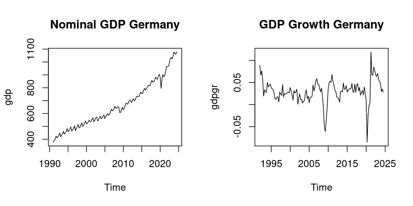
In practice, we are interested in characteristics (parameters) of a population distribution, such as the mean or variance of a variable, or correlations between multiple variables. These characteristics are related to the population moments of a distribution.
While the population distribution and its population moments are unobserved, we can learn about these characteristics using the sample moments of a univariate dataset Y_1, \ldots, Y_n or a multivariate dataset \boldsymbol X_1, \ldots, \boldsymbol X_n. The ideal scenario is that the dataset forms an i.i.d. sample from the underlying population distribution of interest.
The r-th sample moment about the origin (also called the r-th empirical moment) of a univariate sample Y_1, \ldots, Y_n is defined as \overline{Y^r} = \frac{1}{n} \sum_{i=1}^n Y_i^r.
For example, the first sample moment (r=1) is the sample mean (arithmetic mean): \overline Y = \frac{1}{n} \sum_{i=1}^n Y_i. The sample mean is the most common measure of central tendency in a sample.
The population counterpart of the sample mean is the expected value.
The expected value, also called expectation or (population) mean, of a discrete random variable Y with PMF \pi_Y(\cdot) and support \mathcal Y is defined as E[Y] = \sum_{u \in \mathcal Y} u \, \pi_Y(u). The r-th moment (or r-th raw moment) is E[Y^r] = \sum_{u \in \mathcal Y} u^r \, \pi_Y(u).
Suppose the education variable has the following PMF: \pi_Y(a) = P(Y=a) = \begin{cases} 0.008 & \text{if} \ a = 4 \\ 0.048 & \text{if} \ a = 10 \\ 0.392 & \text{if} \ a = 12 \\ 0.072 & \text{if} \ a = 13 \\ 0.155 & \text{if} \ a = 14 \\ 0.071 & \text{if} \ a = 16 \\ 0.225 & \text{if} \ a = 18 \\ 0.029 & \text{if} \ a = 21 \\ 0 & \text{otherwise} \end{cases}
Then, the expected value of education is calculated by summing over all possible values: \begin{align*} E[Y] &= 4\cdot\pi_Y(4) + 10\cdot\pi_Y(10) + 12\cdot \pi_Y(12) \\ &\phantom{=} + 13\cdot\pi_Y(13) + 14\cdot\pi_Y(14) + 16\cdot \pi_Y(16) \\ &\phantom{=} + 18 \cdot \pi_Y(18) + 21 \cdot \pi_Y(21) = 14.117 \end{align*}
A binary random variable Y has support \mathcal Y = \{0,1\}. The probabilities are
for some p \in [0,1]. The expected value of Y is: \begin{align*} E[Y] &=0\cdot\pi_Y(0) + 1\cdot\pi_Y(1) \\ &= 0 \cdot(1-p) + 1 \cdot p \\ &= p. \end{align*} For the variable coin, the probability of heads is p=0.5 and the expected value is E[Y] = p = 0.5.
The expected value of a continuous random variable Y with PDF f_Y(\cdot) is E[Y] = \int_{-\infty}^\infty u \, f_Y(u) \, du. The r-th moment is E[Y^r] = \int_{-\infty}^\infty u^r \, f_Y(u) \, du.
The uniform distribution on the unit interval [0,1] has the PDF f_Y(u) = \begin{cases} 1 & \text{if} \ u \in[0,1], \\ 0 & \text{otherwise,} \end{cases} and the expected value of a uniformly distributed random variable Y is E[Y] = \int_{-\infty}^\infty u\, f_Y(u) \, du = \int_{0}^1 u \, du = \frac{1}{2} u^2 \, \bigg|_0^1= \frac{1}{2}.
Not every distribution has a PMF or a PDF, but every distribution has a CDF. You can define expectation also directly via the CDF using the Riemann-Stieltjes integral: E[Y] = \int_{-\infty}^\infty u \, dF_Y(u). Similarly, the expected value of a function of multiple random variables can be defined via their joint CDF: E[g(Z_1, \ldots, Z_k)] = \int_{\mathbb R^k} g(u_1, \ldots, u_k) \, dF_{Z_1, \ldots, Z_k}(u_1, \ldots, u_k). For more details, see: probability.svenotto.com/part2_expectation.html#general-case
Not every distribution has a well-defined expected value. The simple Pareto distribution with parameter \alpha = 1 has the PDF: f_Y(u) = \begin{cases} \frac{1}{u^2} & \text{if} \ u > 1, \\ 0 & \text{if} \ u \leq 1, \end{cases}
The expected value is: E[Y] = \int_{-\infty}^\infty u f_Y(u) \ \text{d}u = \int_{1}^\infty \frac{u}{u^2} \ \text{d}u = \int_{1}^\infty \frac{1}{u} \ \text{d}u = \log(u)|_1^\infty = \infty, where “= \infty” means it diverges.
The game of chance from the St. Petersburg paradox is a discrete example with infinite expectation. In this game, a fair coin is tossed until a tail appears; if the first tail is on the n-th toss, the payoff is 2^n dollars. The probability of “first tail on the n-th toss” is 2^{-n}. The expected payoff is: E[Y] = \sum_{n=1}^{\infty} 2^n \cdot \frac{1}{2^n} = \sum_{n=1}^{\infty} 1 = \infty
For a t-distributed random variable Y with m degrees of freedom we have E[|Y|^k] < \infty for k < m and E[|Y|^k] = \infty for k \geq m. In particular E[Y] = 0 for m > 1 and E[Y^2] = m/(m-2) for m > 2.
Many statistical procedures require conditions such as E[Y^4] < \infty (finite fourth moments). This excludes distributions with very heavy tails and ensures that large outliers (like extreme payoffs as in the St. Petersburg game) are rare enough.
The sample mean \overline Y is a function of the sample Y_1, \ldots, Y_n and the expected value E[Y] is a function of the population distribution F_Y.
E[Y] is a parameter of the population distribution F_Y. In general, a parameter \theta is a characteristic or feature of a population distribution. Parameters are typically fixed but unknown quantities that we aim to learn about through sampling and estimation.
\overline Y is an estimator for the parameter E[Y]. In general, an estimator \widehat{\theta}_n is a function of sample data intended to approximate the unknown parameter \theta. Since an estimator is a function of random variables (the sample), it is itself a random variable. When we actually compute the estimator from a specific realized sample, we call the resulting value an estimate.
A desired property for any estimator \widehat \theta_n is that it gets closer and closer to the true parameter \theta as the sample size n increases. It eventually converges to the true parameter value in a hypothetically infinitely large sample.
Because \widehat \theta_n is a function of the sample and therefore random, we use convergence in probability rather than a purely deterministic limit.
Convergence in Probability
A sequence of random variables \{W_n\}_{n=1}^{\infty} converges in probability to a constant c if, for any \epsilon > 0, \lim_{n \to \infty} P(|W_n - c| > \epsilon) = 0
Equivalently, this can be expressed as: \lim_{n \to \infty} P(|W_n - c| \leq \epsilon) = 1
This is denoted as W_n \overset{p}{\to} c.
Intuitively, convergence in probability means that as the sample size n increases, the probability that W_n deviates from c by more than any fixed positive amount \epsilon becomes arbitrarily small.
For example, if W_n \overset{p}{\to} c, then for any small \epsilon > 0 (say, \epsilon = 0.01), we can make P(|W_n - c| > 0.01) as small as we want by choosing a sufficiently large sample size n. This doesn’t mean that W_n will exactly equal c for large n, but rather that the probability of W_n being close to c approaches 1 as n grows.
Applying the concept of convergence in probability to an estimator \widehat \theta_n for a parameter \theta leads to the important property of consistency.
Consistency
An estimator \widehat{\theta}_n is consistent for the parameter \theta if: \widehat{\theta}_n \overset{p}{\to} \theta \quad \text{as} \quad n \to \infty
That is, if for any \epsilon > 0: \lim_{n \to \infty} P(|\widehat{\theta}_n - \theta| > \epsilon) = 0
Consistency is a minimal requirement for a good estimator. It ensures that with a large enough sample, the estimator will be arbitrarily close to the true parameter with high probability.
If an estimator \widehat{\theta}_n is a continuous random variable, it will almost never equal exactly the true parameter value because for continuous distributions, point probabilities are zero: P(\widehat{\theta}_n = \theta) = 0.
However, the larger the sample size, the higher the probability that \widehat{\theta}_n falls within a small neighborhood around the true value \theta. Consistency means that, if we fix some small precision value \epsilon > 0, then, P(|\widehat{\theta}_n - \theta| \leq \epsilon) = P(\theta - \epsilon \leq \widehat{\theta}_n \leq \theta + \epsilon) should increase as the sample size n grows, approaching 1 in the limit.
This property aligns with our intuition that more data should lead to better estimates.
The Law of Large Numbers (LLN) is one of the fundamental results in probability theory that establishes the consistency of the sample mean for its population mean.
Law of Large Numbers (LLN)
Let Y_1, Y_2, \ldots, Y_n be a univariate i.i.d. sample with \mu = E[Y_i]. If |\mu| < \infty, then \overline{Y} = \frac{1}{n}\sum_{i=1}^n Y_i \overset{p}{\to} \mu \quad \text{as} \quad n \to \infty.
The LLN essentially states that if we take a large enough sample from a population with finite mean, the sample mean will be close to the population mean with high probability.
Below is an interactive Shiny app to visualize the law of large numbers using simulated data for different sample sizes and different distributions.
The LLN is not confined to i.i.d. data, but for other sampling schemes additional conditions must be satisfied.
Clustered data has the form Y_{gj} for g=1, \ldots, G and j=1, \ldots, n_g. Here, G is the number of clusters and n_g the number of observations in cluster g.
For instance, G may be the number of classrooms, and n_g the number of students in classroom g that take part in a survey (clustered cross section). Or G may be the number of firms and n_g the number of years where the data for firm g is observed (panel data)
The LLN holds for clustered data if
Then, \frac{1}{N} \sum_{g=1}^G \sum_{j=1}^{n_g} Y_{gj} \overset{p}{\to} \mu.
A time series Y_t for t=1, \ldots, n is called (strictly) stationary if the vector (Y_t, Y_{t+1}, \ldots, Y_{t+h})' has the same probability distribution as the vector (Y_{t-j}, Y_{t-j+1}, \ldots, Y_{t-j+h})' for any t, h, and j. That is, the distribution is invariant to time shifts.
For time series data, the LLN \frac{1}{n} \sum_{t=1}^n Y_t \overset{p}{\to} \mu
holds, if
Nominal GDP is typically nonstationary, while year-on-year GDP growth is often (approximately) stationary:
The r-th central sample moment is the average of the r-th powers of the deviations from the sample mean: \frac{1}{n} \sum_{i=1}^n (Y_i - \overline Y)^r For example, the second central moment (r=2) is the sample variance: \widehat \sigma_Y^2 = \frac{1}{n} \sum_{i=1}^n (Y_i - \overline Y)^2 = \overline{Y^2} - \overline Y^2. The sample variance measures the spread or dispersion of the data around the sample mean.
The population variance of a random variable Y is defined as \mathrm{Var}(Y) = E[(Y-E[Y])^2] = E[Y^2] - E[Y]^2.
If Y_1, \ldots, Y_n are i.i.d. draws from the distribution of Y with E[Y^2] < \infty, then \widehat \sigma_Y^2 \overset{p}{\to} \mathrm{Var}(Y).
The sample standard deviation is the square root of the sample variance: \widehat \sigma_Y = \sqrt{\widehat \sigma_Y^2} = \sqrt{\frac{1}{n} \sum_{i=1}^n (Y_i - \overline Y)^2} = \sqrt{\overline{Y^2} - \overline Y^2}. It quantifies the typical deviation of data points from the sample mean in the original units of measurement.
The population standard deviation is \mathrm{sd}(Y) = \sqrt{\mathrm{Var}(Y)}, and \widehat \sigma_Y \overset{p}{\to} \mathrm{sd}(Y) under the same conditions as for the sample variance.
For a bivariate sample (Y_1, Z_1), \ldots, (Y_n, Z_n), we can compute cross moments that describe the relationship between the two variables. The sample cross moment is: \overline{YZ} = \frac{1}{n} \sum_{i=1}^n Y_i Z_i. Under i.i.d. sampling from the distribution of the bivariate random variable (Y,Z), it converges in probability to the population cross moment E[YZ].
The central sample cross moment is also known as the sample covariance and is defined as: \widehat{\sigma}_{YZ} = \frac{1}{n} \sum_{i=1}^n (Y_i - \overline{Y})(Z_i - \overline{Z}) = \overline{YZ} - \overline{Y} \, \overline{Z}. It converges under i.i.d. sampling in probability to the population covariance \mathrm{Cov}(Y,Z) = E[(Y-E[Y])(Z-E[Z])] = E[YZ] - E[Y] E[Z].
The sample correlation coefficient is the standardized sample covariance: r_{YZ} = \frac{\widehat{\sigma}_{YZ}}{\widehat \sigma_Y \widehat \sigma_Z} = \frac{\sum_{i=1}^n (Y_i - \overline{Y})(Z_i - \overline{Z})}{\sqrt{\sum_{i=1}^n (Y_i - \overline{Y})^2}\sqrt{\sum_{i=1}^n (Z_i - \overline{Z})^2}}. Its population counterpart is the population correlation \mathrm{Corr}(Y,Z) = \frac{\mathrm{Cov}(Y,Z)}{\mathrm{sd}(Y) \, \mathrm{sd}(Z)}.
For any random variables X,Y,Z, and real numbers a, b \in \mathbb R, we have the following rules:
The r-th standardized sample moment is the central moment normalized by the sample standard deviation raised to the power of r. It is defined as: \frac{1}{n} \sum_{i=1}^n \bigg(\frac{Y_i - \overline Y}{\widehat \sigma_Y}\bigg)^r, provided that \widehat \sigma_Y > 0.
Its population counterpart is the r-th standardized population moment E\bigg[ \bigg(\frac{Y - E[Y]}{\mathrm{sd}(Y)}\bigg)^r \bigg], provided that \mathrm{sd}(Y) > 0.
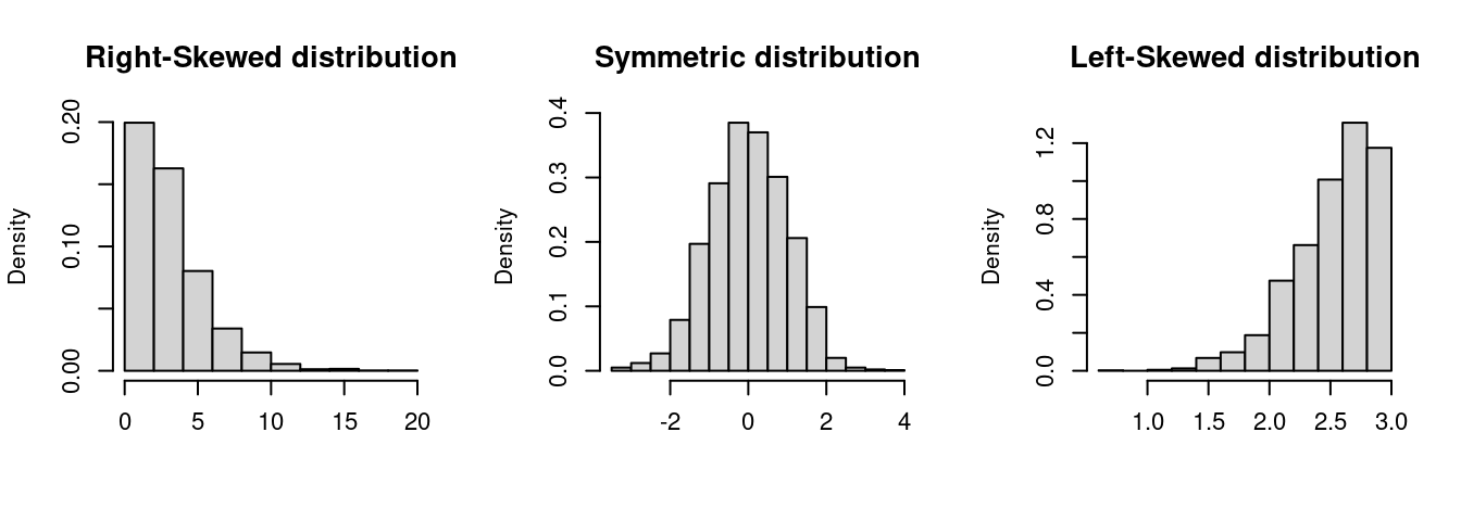
The sample skewness is the third standardized sample moment: \widehat{skew} = \frac{1}{n \widehat \sigma_Y^3} \sum_{i=1}^n (Y_i - \overline Y)^3. The skewness is a measure of asymmetry around the mean. A positive skewness indicates that the distribution has a longer or heavier tail on the right side (right-skewed), while a negative skewness indicates a longer or heavier tail on the left side (left-skewed). A perfectly symmetric distribution, such as the normal distribution, has a skewness of 0.
The population skewness is \mathrm{skew}(Y) = E\bigg[ \bigg(\frac{Y - E[Y]}{\mathrm{sd}(Y)}\bigg)^3 \bigg] = \frac{E[(Y-E[Y])^3]}{\mathrm{sd}(Y)^3}
The sample kurtosis is the fourth standardized sample moment: \widehat{kurt} = \frac{1}{n \widehat \sigma_Y^4} \sum_{i=1}^n (Y_i - \overline Y)^4.
Kurtosis measures the “tailedness” or heaviness of the tails of a distribution and can indicate the presence of extreme outliers. The reference value of kurtosis is 3, which corresponds to the kurtosis of a normal distribution. Values greater than 3 suggest heavier tails, while values less than 3 indicate lighter tails.
The population kurtosis is \mathrm{kurt}(Y) = E\bigg[ \bigg(\frac{Y - E[Y]}{\mathrm{sd}(Y)}\bigg)^4 \bigg] = \frac{E[(Y-E[Y])^4]}{\mathrm{Var}(Y)^2}.
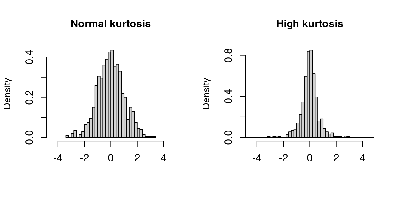
The plots display histograms of two standardized datasets (both have a sample mean of 0 and a sample variance of 1). The left dataset has a normal sample kurtosis (around 3), while the right dataset has a high sample kurtosis with heavier tails.
Let’s load the CPS dataset from Section 1:
cps = read.csv("cps.csv")
par(mfrow = c(1,2))
hist(cps$experience, probability = TRUE)
hist(cps$wage, probability = TRUE)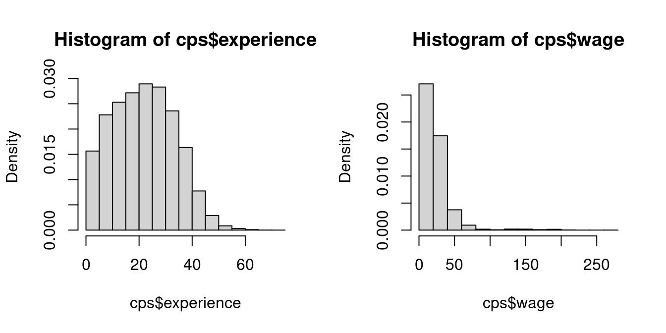
To compute the sample skewness and kurtosis we can use the moments package
Wages are right-skewed because a few very rich individuals earn much more than the many with low to medium incomes. Experience does not indicate any pronounced skewness.
Wages have a large kurtosis due to a few super-rich individuals in the sample. The kurtosis of experience is close to 3 and thus similar to a normal distribution.
Right-skewed, heavy-tailed variables are common in real-world datasets, such as income levels, wealth accumulation, property values, insurance claims, and social media follower counts. A common transformation to reduce skewness and kurtosis in data is to use the natural logarithm:
par(mfrow = c(1,2))
hist(cps$wage, probability = TRUE, breaks = 20)
hist(log(cps$wage), probability = TRUE, breaks = 50, xlim = c(-1, 6))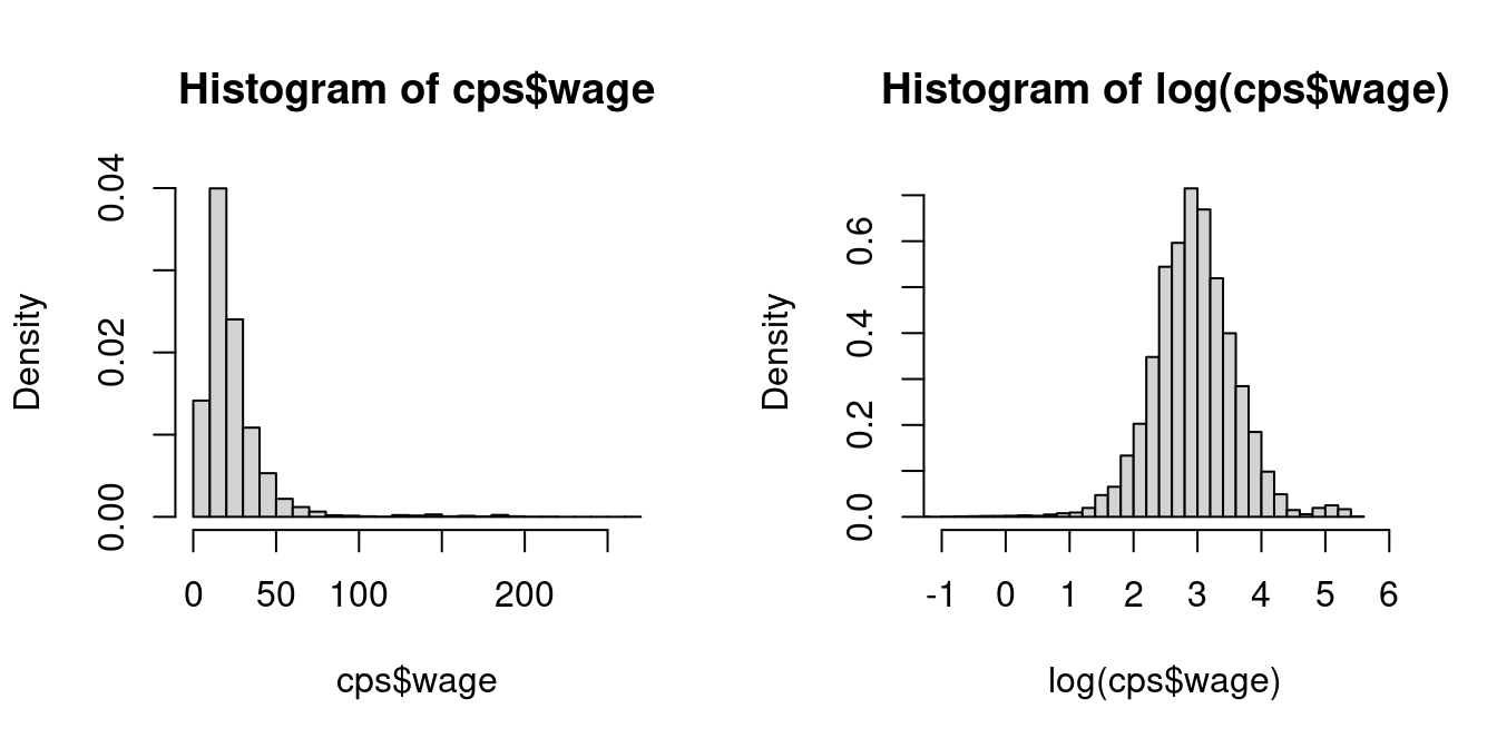
In econometrics, statistics, and many programming languages including R, \log(\cdot) is commonly used to denote the natural logarithm (base e).
Note: On a pocket calculator, use LN to calculate the natural logarithm \log(\cdot)=\log_e(\cdot). If you use LOG, you will calculate the logarithm with base 10, i.e., \log_{10}(\cdot), which will give you a different result. The relationship between these logarithms is \log_{10}(x) = \log_{e}(x)/\log_{e}(10).
Consider a multivariate i.i.d. dataset \boldsymbol X_1, \ldots, \boldsymbol X_n with \boldsymbol X_i = (X_{i1}, \ldots, X_{ik})', such as the following subset of the cps dataset:
dat = data.frame(wage = cps$wage, education = cps$education, female = cps$female)The sample mean vector \overline{\boldsymbol X} contains the sample means of the k variables and is defined as \overline{\boldsymbol X} = \frac{1}{n} \sum_{i=1}^n \boldsymbol X_i = \frac{1}{n} \sum_{i=1}^n \begin{pmatrix} X_{i1} \\ \vdots \\ X_{ik} \end{pmatrix}.
Its population counterpart is the population mean vector E[\boldsymbol X_i] = E[(X_{i1},\ldots, X_{ik})']
The sample cross-moment matrix is \frac{1}{n} \sum_{i=1}^n \boldsymbol X_i \boldsymbol X_i' = \frac{1}{n} \sum_{i=1}^n \begin{pmatrix} X_{i1}^2 & X_{i1} X_{i2} & \ldots & X_{i1} X_{ik} \\ X_{i1} X_{i2} & X_{i2}^2 & \ldots & X_{i2} X_{ik} \\ \vdots & \vdots & \ddots & \vdots \\ X_{i1} X_{ik} & X_{i2} X_{ik} & \ldots & X_{ik}^2 \end{pmatrix}
Its population counterpart is E[\boldsymbol X_i \boldsymbol X_i'].
The sample covariance matrix \widehat{\Sigma} is the k \times k matrix given by \widehat{\Sigma} = \frac{1}{n} \sum_{i=1}^n (\boldsymbol X_i - \overline{\boldsymbol X})(\boldsymbol X_i - \overline{\boldsymbol X})'. Its elements \widehat \sigma_{h,l} represent the pairwise sample covariance between variables h and l: \widehat \sigma_{h,l} = \frac{1}{n} \sum_{i=1}^n (X_{ih} - \overline{X_h})(X_{il} - \overline{X_l}), \quad \overline{X_h} = \frac{1}{n} \sum_{i=1}^n X_{ih}.
The population counterpart is the population covariance matrix: \begin{align*} \mathrm{Var}(\boldsymbol X_i) &= E[(\boldsymbol X_i - E[\boldsymbol X_i])(\boldsymbol X_i - E[\boldsymbol X_i])'] \\ &= E[\boldsymbol X_i \boldsymbol X_i'] - E[\boldsymbol X_i] E[\boldsymbol X_i]'. \end{align*}
The sample correlation coefficient between the variables h and l is the standardized sample covariance: r_{h,l} = \frac{\widehat \sigma_{h,l}}{\widehat \sigma_h \widehat \sigma_l} = \frac{\sum_{i=1}^n (X_{ih} - \overline{X_h})(X_{il} - \overline{X_l})}{\sqrt{\sum_{i=1}^n (X_{ih} - \overline{X_h})^2}\sqrt{\sum_{i=1}^n (X_{il} - \overline{X_l})^2}}. These coefficients form the sample correlation matrix R, expressed as:
R = D^{-1} \widehat{\Sigma} D^{-1}, where D is the diagonal matrix of sample standard deviations: D = \mathrm{diag}(\widehat \sigma_1, \ldots, \widehat \sigma_k) = \begin{pmatrix} \widehat \sigma_1 & 0 & \ldots & 0 \\ 0 & \widehat \sigma_2 & \ldots & 0 \\ \vdots & & \ddots & \vdots \\ 0 & 0 & \ldots & \widehat \sigma_k \end{pmatrix} The covariance and correlation matrices are symmetric and positive semidefinite.
cor(dat) wage education female
wage 1.0000000 0.38398973 -0.16240519
education 0.3839897 1.00000000 0.04448972
female -0.1624052 0.04448972 1.00000000We find a strong positive correlation between wage and education, a substantial negative correlation between wage and female, and a negligible correlation between education and female.