| person | wage | education | female |
|---|---|---|---|
| 1 | 10.40 | 12 | 0 |
| 2 | 18.68 | 16 | 0 |
| 3 | 12.44 | 14 | 1 |
| 4 | 54.73 | 18 | 0 |
| 5 | 24.27 | 14 | 0 |
| 6 | 24.41 | 12 | 1 |
1 Data
1.1 Data Structures
Univariate Datasets
A univariate dataset consists of a sequence of observations: Y_1, \ldots, Y_n. These n observations form a data vector: \boldsymbol{Y} = (Y_1, \ldots, Y_n)'.
Example: Survey of six individuals on their hourly earnings. Data vector: \boldsymbol{Y} = \begin{pmatrix} 10.40 \\ 18.68 \\ 12.44 \\ 54.73 \\ 24.27 \\ 24.41 \end{pmatrix}.
Multivariate Datasets
Typically, we have data on more than one variable, such as years of education and gender. Categorical variables are often encoded as dummy variables (also called indicator variables), which are binary variables. The female dummy variable is defined as: D_i = \begin{cases} 1 & \text{if person } i \text{ is female,} \\ 0 & \text{otherwise.} \end{cases}
A k-variate dataset (or multivariate dataset) is a collection of n observations on k variables (i.e., n observation vectors of length k): \boldsymbol{X}_1, \ldots, \boldsymbol{X}_n.
The i-th vector contains the data on all k variables for individual i: \boldsymbol{X}_i = (X_{i1}, \ldots, X_{ik})'.
Thus, X_{ij} represents the value for the j-th variable of individual i. The full k-variate dataset is structured in the n \times k data matrix \boldsymbol{X}: \boldsymbol{X} = \begin{pmatrix} \boldsymbol{X}_1' \\ \vdots \\ \boldsymbol{X}_n' \end{pmatrix} = \begin{pmatrix} X_{11} & \ldots & X_{1k} \\ \vdots & \ddots & \vdots \\ X_{n1} & \ldots & X_{nk} \end{pmatrix}
The i-th row in \boldsymbol{X} corresponds to the values from \boldsymbol{X}_i. Since \boldsymbol{X}_i is a column vector, we write rows of the data matrix as \boldsymbol{X}_i' (its transpose), which is a row vector. Note that \boldsymbol X \in \mathbb R^{n \times k}, \boldsymbol X_i \in \mathbb R^{k \times 1}, and \boldsymbol X_i' \in \mathbb R^{1 \times k}.
The data matrix for our example is: \boldsymbol X = \begin{pmatrix} 10.40 & 12 & 0 \\ 18.68 & 16 & 0 \\ 12.44 & 14 & 1 \\ 54.73 & 18 & 0 \\ 24.27 & 14 & 0 \\ 24.41 & 12 & 1 \end{pmatrix}
with data vectors: \begin{align*} \boldsymbol X_1 &= \begin{pmatrix} 10.40 \\ 12 \\ 0 \end{pmatrix} \\ \boldsymbol X_2 &= \begin{pmatrix} 18.68 \\ 16 \\ 0 \end{pmatrix} \\ \boldsymbol X_3 &= \begin{pmatrix} 12.44 \\ 14 \\ 1 \end{pmatrix} \\ & \ \ \vdots \end{align*}
Matrix Algebra
Vector and matrix algebra provide a compact mathematical representation of multivariate data and an efficient framework for analyzing and implementing statistical methods. We will use matrix algebra frequently throughout this course.
To refresh or enhance your knowledge of matrix algebra, consult the following resources:
Crash Course on Matrix Algebra:
matrix.svenotto.com (in particular Sections 1-3)
Section 19.1 of the Stock and Watson textbook also provides a brief overview of matrix algebra concepts.
1.2 Datasets in R
R is a vector-based statistical programming language and is therefore particularly suitable for handling data in tabular or matrix form. Matrix algebra is particularly useful when working with real data in R.
R’s most common data structure for tabular data is the data frame (data.frame). Like the data matrix \boldsymbol{X} we defined earlier, it organizes data with variables as columns and observations as rows.
CA Schools Data
Let’s load the CASchools dataset from the AER package (“Applied Econometrics with R”). You can install the package with the command install.packages("AER").
data(CASchools, package = "AER")The dataset is used throughout Sections 4–8 of Stock and Watson’s textbook Introduction to Econometrics. It was collected in 1998 and captures California school characteristics including test scores, teacher salaries, student demographics, and district-level metrics.
| Variable | Description | Variable | Description |
|---|---|---|---|
| district | District identifier | lunch | % receiving free meals |
| school | School name | computer | Number of computers |
| county | County name | expenditure | Spending per student ($) |
| grades | Through 6th or 8th | income | District avg income ($000s) |
| students | Total enrollment | english | Non-native English (%) |
| teachers | Teaching staff | read | Average reading score |
| calworks | % CalWorks aid | math | Average math score |
The Environment pane in RStudio’s top-right corner displays all objects currently in your workspace, including the CASchools dataset. You can click on it to explore its contents.
The head() function displays the first few rows of a dataset, giving you a quick preview of its content.
head(CASchools) district school county grades students teachers
1 75119 Sunol Glen Unified Alameda KK-08 195 10.90
2 61499 Manzanita Elementary Butte KK-08 240 11.15
3 61549 Thermalito Union Elementary Butte KK-08 1550 82.90
4 61457 Golden Feather Union Elementary Butte KK-08 243 14.00
5 61523 Palermo Union Elementary Butte KK-08 1335 71.50
6 62042 Burrel Union Elementary Fresno KK-08 137 6.40
calworks lunch computer expenditure income english read math
1 0.5102 2.0408 67 6384.911 22.690001 0.000000 691.6 690.0
2 15.4167 47.9167 101 5099.381 9.824000 4.583333 660.5 661.9
3 55.0323 76.3226 169 5501.955 8.978000 30.000002 636.3 650.9
4 36.4754 77.0492 85 7101.831 8.978000 0.000000 651.9 643.5
5 33.1086 78.4270 171 5235.988 9.080333 13.857677 641.8 639.9
6 12.3188 86.9565 25 5580.147 10.415000 12.408759 605.7 605.4The variable students contains the total number of students enrolled in a school. It is the fifth variable in the dataset. To access the variable as a vector, you can type CASchools[,5] (the fifth column in your data matrix), CASchools[,"students"], or simply CASchools$students.
We can easily add new variables to our data frame, for instance, the student-teacher ratio (the total number of students per teacher) and the average test score (average of the math and reading scores):
# compute student-teacher ratio and append it to CASchools
CASchools$STR = CASchools$students/CASchools$teachers
# compute test score and append it to CASchools
CASchools$score = (CASchools$read + CASchools$math)/2
Scatterplots provide further insights:
par(mfrow = c(1,3))
plot(score~STR, data = CASchools)
plot(score~income, data = CASchools)
plot(score~english, data = CASchools)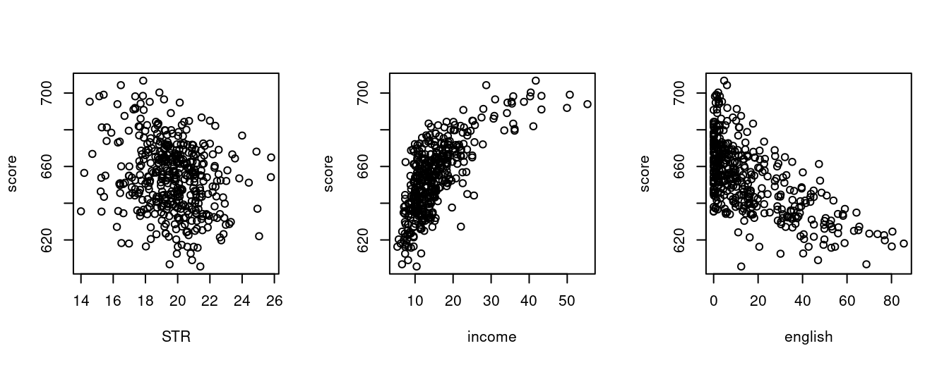
The option par(mfrow = c(1,3)) allows you to display multiple plots side by side. Try what happens if you replace c(1,3) with c(3,1).
CPS Data
Another dataset we will use in this course is the CPS dataset from Bruce Hansen’s textbook Econometrics.
The Current Population Survey (CPS) is a monthly survey conducted by the U.S. Census Bureau for the Bureau of Labor Statistics, primarily used to measure the labor force status of the U.S. population.
- Dataset: cps09mar.txt
- Codebook: cps09mar_description.pdf
The dataset is available as a whitespace-separated text file, which can be loaded using read.table().
url = "https://users.ssc.wisc.edu/~bhansen/econometrics/cps09mar.txt"
varnames = c("age", "female", "hisp", "education", "earnings", "hours",
             "week", "union", "uncov", "region", "race", "marital")
cps = read.table(url, col.names = varnames)
Let’s create additional variables:
# wage per hour
cps$wage = cps$earnings/(cps$week * cps$hours)
# work experience (years since graduation)
cps$experience = pmax(cps$age - cps$education - 6,0)
# married dummy (see codebook for the categories)
cps$married = (cps$marital %in% c(1, 2, 3)) |> as.numeric()
# Black dummy (see codebook)
cps$Black = (cps$race %in% c(2, 6, 10, 11, 12, 15, 16, 19)) |> as.numeric()
# Asian dummy (see codebook)
cps$Asian = (cps$race %in% c(4, 8, 11, 13, 14, 16, 17, 18, 19)) |> as.numeric()
A person is considered married if the marital variable takes one of the following categories: 1, 2, or 3 (see the codebook above for more information). Note that cps$marital %in% c(1, 2, 3) is a logical expression with either TRUE or FALSE values. The command as.numeric() creates a dummy variable by translating TRUE to 1 and FALSE to 0.
The pipe operator |> efficiently chains commands. It passes the output of one function as the input to another. For example, cps$marital %in% c(1, 2, 3) |> as.numeric() gives the same output as as.numeric(cps$marital %in% c(1, 2, 3)).
We will need the CPS dataset later, so it is a good idea to save the dataset to your computer:
write.csv(cps, "cps.csv", row.names = FALSE)This command saves the dataset to a file named cps.csv in your current working directory. It’s best practice to use an R Project for your course work so that all files (data, scripts, outputs) are stored in a consistent and organized folder structure.
To read the data back into R later, just type cps = read.csv("cps.csv").
1.3 Statistical Framework
Data are usually the result of a random experiment. The gender of the next person you meet, the daily fluctuation of a stock price, the monthly music streams of your favorite artist, the annual number of pizzas consumed - all of this information involves a certain amount of randomness.
We distinguish between:
- Cross-sectional data: observations on many units at (approximately) one point in time.
- Time series data: observations on one unit recorded over multiple time periods.
- Panel data: observations on many units recorded over multiple time periods.
In statistical sciences, we interpret a univariate dataset Y_1, \ldots, Y_n as a sequence of random variables. Similarly, a multivariate dataset \boldsymbol X_1, \ldots, \boldsymbol X_n is viewed as a sequence of random vectors.
Sampling refers to the process of obtaining data by drawing observations from a population, which is often considered infinite in statistical theory. An infinite population is a conceptual device representing all potential outcomes that could arise under the same conditions, not just the currently existing individuals.
For example, when modeling coin flips, the population includes every possible toss that could ever occur. When analyzing stock returns, the population includes all possible future price movements. When studying human height, the infinite population includes all current humans as well as all hypothetical humans who could exist under similar biological conditions. Formally, the infinite population corresponds to a probability distribution F and the sample is n i.i.d. draws from F.
Random sampling
Econometric methods require specific assumptions about sampling processes. The ideal approach for a cross-sectional study is simple random sampling, where each individual from the population has an equal chance of being selected independently.
This produces observations \boldsymbol X_1, \ldots, \boldsymbol X_n that are both identically distributed (drawn from the same population) and independently drawn (as if drawn from an urn with replacement). We call these data independent and identically distributed (i.i.d.) or simply a random sample.
For example, when conducting a representative survey, the answers of the second randomly selected individual should not depend on the answers of the first randomly selected individual if the individuals are truly randomly selected from the population. A violation of the i.i.d. property is often a matter of data collection quality.
Clustered sampling
While i.i.d. sampling provides a clean theoretical foundation, real-world data sometimes exhibit clustering - where observations are naturally grouped or nested within larger units. This clustering leads to dependencies that violate the i.i.d. assumption:
In cross-sectional studies, clustering occurs when we collect data on individual units that belong to distinct groups. Consider a study on student achievement where researchers randomly select schools, then collect data from all students within those schools:
- Although schools might be selected independently, observations at the student level are dependent
- Students within the same school share common environments (facilities, resources, administration)
- They experience similar teaching quality and educational policies and they influence each other through peer effects and social interactions
For instance, if School A has an exceptional mathematics department, all students from that school may perform better in math tests compared to students with similar abilities in other schools.
Panel data, by its very nature, introduces clustering across both cross-sectional units and time. If many randomly selected individuals are interviewed over many years, then the observations of two different individuals are independent but, for each individual, observations across different years are dependent due to persistent personal factors.
Time dependence
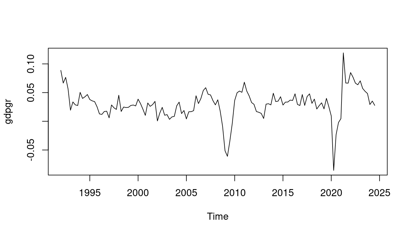
Time series and panel data are intrinsically not independent due to the sequential nature of the observations. We usually expect observations close in time to be strongly dependent and observations at greater temporal distances to be less dependent.
Consider the quarterly GDP growth rates for Germany in the dataset gdpgr. Unlike cross-sectional data where the ordering of observations is arbitrary, the chronological ordering in time series carries crucial information about the dependency structure.