6 Inference
Section 5 interpreted estimated regression coefficients and effects.
A different sample from the same population would generally give different estimates.
Statistical inference quantifies this sampling uncertainty.
The three ingredients of inference are:
- A point estimate is a single estimate of the unknown population parameter.
- A standard error measures the sampling uncertainty of the estimate.
- A critical value is chosen from the approximating distribution.
This section uses these ingredients to construct confidence intervals.
Hypothesis tests follow in Section 7.
6.1 Estimation Uncertainty
Let \widehat\theta_n estimate a population parameter \theta from an i.i.d. sample of size n.
The sampling distribution of \widehat\theta_n describes the estimates obtained from all possible samples of this size.
Its standard deviation \mathrm{sd}(\widehat\theta_n) measures how much the estimator varies across repeated samples.
This quantity is generally unknown.
Standard Error
A standard error estimates the standard deviation of an estimator using the observed sample.
It measures the estimator’s sampling uncertainty.
Example: The Sample Mean
For an i.i.d. sample with 0<\mathrm{Var}(Y_i)=\sigma_Y^2<\infty, the variance rules from Section 3 give \begin{aligned} \mathrm{Var}(\overline Y_n) &=\mathrm{Var}\!\left(\frac1n\sum_{i=1}^nY_i\right)\\ &=\frac1{n^2}\sum_{i=1}^n\mathrm{Var}(Y_i) =\frac{\sigma_Y^2}{n}. \end{aligned}
The second equality holds by independence. Taking square roots gives \mathrm{sd}(\overline Y_n)=\frac{\sigma_Y}{\sqrt n}.
Replacing \sigma_Y by the sample standard deviation gives the standard error \mathrm{se}(\overline Y_n) =\frac{\widehat\sigma_Y}{\sqrt n}, \qquad \widehat\sigma_Y^2 =\frac1n\sum_{i=1}^n(Y_i-\overline Y_n)^2.
- The standard deviation of Y_i describes the dispersion of Y_i across individuals.
- The standard deviation of \overline Y_n describes the dispersion of sample means across samples.
- The standard error of \overline Y_n estimates the standard deviation of \overline Y_n.
In this example, \frac{\mathrm{se}(\overline Y_n)} {\mathrm{sd}(\overline Y_n)} =\frac{\widehat\sigma_Y}{\sigma_Y} \overset{p}{\to}1.
For regression, we use a large-sample approximation to the sampling distribution. The standard error estimates the standard deviation of this approximating distribution.
6.2 Normal Distribution
The normal distribution is also called the Gaussian distribution.
Normal Distribution
A random variable Y has a normal distribution if its PDF is f_Y(y) = \frac{1}{\sqrt{2\pi\sigma^2}} \exp\left( -\frac{(y-\mu)^2}{2\sigma^2} \right), \qquad y\in\mathbb R.
We write Y\sim\mathcal N(\mu,\sigma^2), where \mu\in\mathbb R and \sigma^2>0. Its mean and variance are E[Y]=\mu, \qquad \mathrm{Var}(Y)=\sigma^2.
The mean determines the center of the distribution. The variance determines its dispersion.
The normal distribution with mean zero and variance one is the standard normal distribution: Z\sim\mathcal N(0,1).
Let \phi denote its PDF and let \Phi denote its CDF.
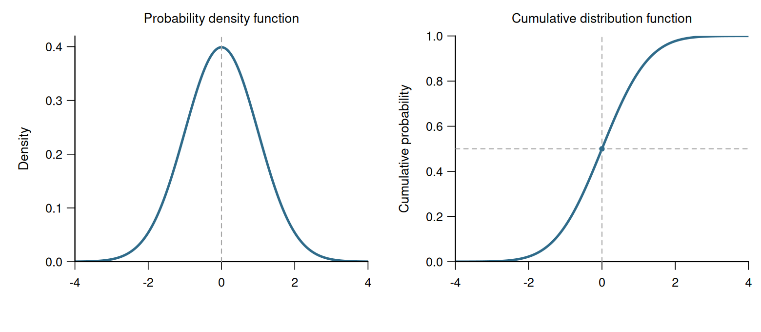
Symmetry implies \phi(a)=\phi(-a), \qquad \Phi(-a)=1-\Phi(a). \tag{6.1}
Thus, intervals and tail probabilities can be calculated symmetrically around zero.
Every normal variable can be standardized: Y\sim\mathcal N(\mu,\sigma^2) \quad\Longrightarrow\quad \frac{Y-\mu}{\sigma}\sim\mathcal N(0,1).
Quantiles
For 0<p<1, the p-quantile is the value at which the CDF first reaches or exceeds p.
Thus, at least a fraction p of the population lies at or below this value. The 0.5-quantile is the median.
For a continuous, strictly increasing CDF F_Y, the p-quantile q_p satisfies F_Y(q_p)=p.
For the standard normal distribution, we write z_p=\Phi^{-1}(p), \qquad P(Z\leq z_p)=\Phi(z_p)=p.
Some important standard normal quantiles are:
| p | 0.90 | 0.95 | 0.975 | 0.99 | 0.995 |
|---|---|---|---|---|---|
| z_p | 1.282 | 1.645 | 1.960 | 2.326 | 2.576 |
In particular, \Phi(1.96)=0.975 and, by symmetry, \Phi(-1.96)=0.025.
Therefore, P(-1.96\leq Z\leq1.96) =0.975-0.025=0.95.
Multivariate Normal Distribution
A random vector \boldsymbol V is multivariate normal if each nonconstant linear combination of its components is normally distributed.
We write \boldsymbol V\sim\mathcal N(\boldsymbol\mu,\boldsymbol\Sigma), where E[\boldsymbol V]=\boldsymbol\mu, \qquad \mathrm{Var}(\boldsymbol V)=\boldsymbol\Sigma.
The components may be dependent. Their variances and covariances are collected in \boldsymbol\Sigma.
6.3 Central Limit Theorem
Let F_{V_n} be the CDF of V_n and let F_V be the CDF of V.
We say that V_n converges in distribution to V, written V_n\overset{d}{\to}V, if \lim_{n\to\infty}F_{V_n}(a)=F_V(a) at every value a where F_V is continuous.
Thus, the CDF of V_n approaches the CDF of V at its continuity points.
In particular, V_n\overset{d}{\to}\mathcal N(0,1) \quad\Longrightarrow\quad P(V_n\leq a)\longrightarrow\Phi(a) for every a\in\mathbb R.
Univariate Central Limit Theorem (CLT)
Let Y_1,Y_2,\ldots be i.i.d. with E[Y_i]=\mu, \qquad 0<\mathrm{Var}(Y_i)=\sigma_Y^2<\infty.
Then \sqrt n(\overline Y_n-\mu) \overset{d}{\to}\mathcal N(0,\sigma_Y^2). \tag{6.2}
Equivalently, \frac{\overline Y_n-\mu}{\sigma_Y/\sqrt n} \overset{d}{\to}\mathcal N(0,1).
The standard deviation of \overline Y_n-\mu converges to zero at rate 1/\sqrt n.
Multiplying the estimation error \overline Y_n-\mu by \sqrt n compensates for this decrease and keeps its fluctuations on a constant scale.
The normal approximation concerns the distribution of sample means across repeated samples; the individual observations need not be normally distributed.
The LLN from Section 3 shows that the sample mean \overline Y_n approaches \mu.
The CLT additionally describes the rate and the approximate shape of its sampling distribution.
For a large sample, \overline Y_n \overset{\mathrm{approx.}}{\sim} \mathcal N\left(\mu,\frac{\sigma_Y^2}{n}\right).
The sampling distribution is approximately normal, with a standard deviation proportional to 1/\sqrt n.
Increasing the sample size by a factor of four reduces the standard deviation of the sample mean by a factor of two.
The same theorem applies to averages of transformed observations, such as Y_i^2 or Z_iY_i, provided its assumptions hold.
Multivariate Central Limit Theorem
Let \boldsymbol W_1,\boldsymbol W_2,\ldots be i.i.d. k-dimensional random vectors, where k is fixed.
Assume each component of \boldsymbol W_i has a finite second moment. Write \boldsymbol\theta=E[\boldsymbol W_i], \qquad \boldsymbol\Omega=\mathrm{Var}(\boldsymbol W_i).
For the sample mean \overline{\boldsymbol W}_n :=\frac1n\sum_{i=1}^n\boldsymbol W_i, we have \sqrt n\left( \overline{\boldsymbol W}_n -\boldsymbol\theta \right) \overset{d}{\to}\mathcal N(\boldsymbol 0,\boldsymbol\Omega). \tag{6.3}
The limiting distribution is multivariate normal, with mean vector \boldsymbol 0 and covariance matrix \boldsymbol\Omega.
The components of \boldsymbol W_i within an observation may be dependent. Their covariances enter \boldsymbol\Omega.
6.4 Asymptotic Normality of OLS
Consider the exact linear CEF from Section 4: Y_i=\boldsymbol X_i'\boldsymbol\beta+u_i, \qquad E[u_i\mid\boldsymbol X_i]=0.
Recall the population and sample second-moment matrices \boldsymbol Q=E[\boldsymbol X_i\boldsymbol X_i'], \qquad \widehat{\boldsymbol Q} =\frac{1}{n}\sum_{i=1}^n \boldsymbol X_i\boldsymbol X_i'.
Substituting the regression equation into the OLS estimator gives \begin{aligned} \widehat{\boldsymbol\beta} &=\widehat{\boldsymbol Q}^{-1} \frac{1}{n}\sum_{i=1}^n\boldsymbol X_i Y_i \\ &=\widehat{\boldsymbol Q}^{-1} \frac{1}{n}\sum_{i=1}^n \boldsymbol X_i(\boldsymbol X_i'\boldsymbol\beta+u_i) \\ &=\widehat{\boldsymbol Q}^{-1}\widehat{\boldsymbol Q}\boldsymbol\beta +\widehat{\boldsymbol Q}^{-1} \frac{1}{n}\sum_{i=1}^n\boldsymbol X_i u_i \\ &=\boldsymbol\beta+\widehat{\boldsymbol Q}^{-1} \frac{1}{n}\sum_{i=1}^n\boldsymbol X_i u_i. \end{aligned}
Subtracting \boldsymbol\beta and multiplying by \sqrt n gives \sqrt n(\widehat{\boldsymbol\beta}-\boldsymbol\beta) =\widehat{\boldsymbol Q}^{-1} \frac{1}{\sqrt n}\sum_{i=1}^n\boldsymbol X_i u_i. \tag{6.4}
Define \boldsymbol\Omega :=E[u_i^2\boldsymbol X_i\boldsymbol X_i'].
Because E[\boldsymbol X_i u_i]=\boldsymbol 0, the covariance matrix of the moment vector \boldsymbol X_i u_i is \begin{aligned} \mathrm{Var}(\boldsymbol X_i u_i) &=E[(\boldsymbol X_i u_i)(\boldsymbol X_i u_i)'] -E[\boldsymbol X_i u_i]E[\boldsymbol X_i u_i]' \\ &=E[u_i^2\boldsymbol X_i\boldsymbol X_i'] =\boldsymbol\Omega. \end{aligned}
For simple regression, the moment vector has two entries: \boldsymbol X_i=(1,Z_i)' \quad\Longrightarrow\quad \boldsymbol X_i u_i= \begin{pmatrix}u_i\\ Z_i u_i\end{pmatrix}.
Apply the multivariate CLT in Equation 6.3 to \boldsymbol W_i=\boldsymbol X_i u_i, whose mean is \boldsymbol 0.
Its finite-second-moment condition requires E[X_{ij}^2u_i^2]<\infty for every regressor. This is stronger than the moment conditions used for consistency alone.
One sufficient condition is that the regressors and the error have finite fourth moments: E[X_{ij}^4]<\infty\quad\text{for every }j, \qquad E[u_i^4]<\infty.
Applying the Cauchy–Schwarz inequality to X_{ij}^2 and u_i^2 gives E[X_{ij}^2u_i^2] \leq\sqrt{E[X_{ij}^4]E[u_i^4]} <\infty.
Finite fourth moments are sufficient, but not necessary. The CLT requires finite second moments of the products X_{ij}u_i.
Under the conditions below, the LLN and multivariate CLT give the two limits in Equation 6.4: \sqrt n(\widehat{\boldsymbol\beta}-\boldsymbol\beta) = \underbrace{\widehat{\boldsymbol Q}^{-1}} _{\overset{p}{\to}\,\boldsymbol Q^{-1}} \underbrace{\frac{1}{\sqrt n}\sum_{i=1}^n\boldsymbol X_i u_i} _{\overset{d}{\to}\,\mathcal N(\boldsymbol 0,\boldsymbol\Omega)}.
For a fixed matrix \boldsymbol A, a normal vector transforms as \boldsymbol V\sim\mathcal N(\boldsymbol 0,\boldsymbol\Omega) \quad\Longrightarrow\quad \boldsymbol A\boldsymbol V \sim\mathcal N(\boldsymbol 0,\boldsymbol A\boldsymbol\Omega\boldsymbol A').
Taking \boldsymbol A=\boldsymbol Q^{-1} gives \mathrm{Var}(\boldsymbol Q^{-1}\boldsymbol V) =\boldsymbol Q^{-1}\boldsymbol\Omega(\boldsymbol Q^{-1})' =\boldsymbol Q^{-1}\boldsymbol\Omega\boldsymbol Q^{-1}, because \boldsymbol Q^{-1} is symmetric.
Combining these steps gives the following result.
Asymptotic Normality of OLS
Suppose the exact linear CEF is correctly specified: Y_i=\boldsymbol X_i'\boldsymbol\beta+u_i, \qquad E[u_i\mid\boldsymbol X_i]=0.
Assume:
- (Y_i,\boldsymbol X_i')' are i.i.d.,
- \boldsymbol Q and \boldsymbol\Omega have finite entries,
- and \boldsymbol Q is invertible.
Then \sqrt n(\widehat{\boldsymbol\beta}-\boldsymbol\beta) \overset{d}{\to} \mathcal N(\boldsymbol 0,\boldsymbol\Sigma_\beta), \tag{6.5} where \boldsymbol\Sigma_\beta =\boldsymbol Q^{-1}\boldsymbol\Omega\boldsymbol Q^{-1}.
Thus, for a large sample, \widehat{\boldsymbol\beta} \overset{\mathrm{approx.}}{\sim} \mathcal N\left( \boldsymbol\beta, \frac{1}{n}\boldsymbol\Sigma_\beta \right).
The matrix \boldsymbol\Sigma_\beta is the covariance matrix of the limiting distribution in Equation 6.5.
The approximate covariance matrix of \widehat{\boldsymbol\beta} is \boldsymbol\Sigma_\beta/n.
6.5 Robust Standard Errors
The conditional variance measures dispersion around the conditional mean: \mathrm{Var}(Y\mid\boldsymbol X) :=E\!\left[(Y-E[Y\mid\boldsymbol X])^2\mid\boldsymbol X\right].
Because E[u_i\mid\boldsymbol X_i]=0, the conditional error variance is \sigma^2(\boldsymbol x) :=\mathrm{Var}(u_i\mid\boldsymbol X_i=\boldsymbol x) =E[u_i^2\mid\boldsymbol X_i=\boldsymbol x].
The errors are homoskedastic if this variance is constant. Then E[u_i^2\mid\boldsymbol X_i=\boldsymbol x]=\sigma^2 for every i and regressor value \boldsymbol x.
They are heteroskedastic if it changes with \boldsymbol x.
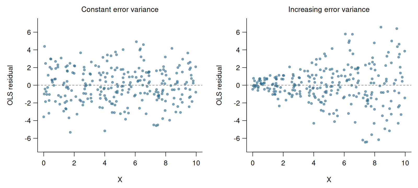
The residuals illustrate a roughly constant spread on the left and an increasing spread on the right.
In the general case, \boldsymbol\Omega =E[u_i^2\boldsymbol X_i\boldsymbol X_i'] =E[\sigma^2(\boldsymbol X_i) \boldsymbol X_i\boldsymbol X_i'].
Here, \sigma^2(\boldsymbol X_i)=\mathrm{Var}(u_i\mid\boldsymbol X_i) = E[u_i^2\mid\boldsymbol X_i].
We do not need to assume homoskedasticity to estimate \boldsymbol\Omega.
HC0 Covariance Matrix
If the population errors were observable, the LLN would give \frac1n\sum_{i=1}^n u_i^2\boldsymbol X_i\boldsymbol X_i' \overset{p}{\to} E[u_i^2\boldsymbol X_i\boldsymbol X_i'] =\boldsymbol\Omega.
The OLS residual satisfies \widehat u_i =Y_i-\boldsymbol X_i'\widehat{\boldsymbol\beta} =u_i-\boldsymbol X_i' (\widehat{\boldsymbol\beta}-\boldsymbol\beta).
OLS is consistent under the maintained sampling and moment assumptions.
Therefore, when replacing errors by residuals, the effect of the additional term \boldsymbol X_i'(\widehat{\boldsymbol\beta}-\boldsymbol\beta) on this weighted sample average vanishes as n grows.
Consequently, the residual-based estimator satisfies \widehat{\boldsymbol\Omega}_{HC0} :=\frac{1}{n}\sum_{i=1}^n \widehat u_i^2\boldsymbol X_i\boldsymbol X_i' \overset{p}{\to}\boldsymbol\Omega.
HC0 Covariance Matrix
The resulting heteroskedasticity-consistent covariance matrix estimator is \widehat{\mathrm{Var}}_{HC0} (\widehat{\boldsymbol\beta}) :=\frac{1}{n} \widehat{\boldsymbol Q}^{-1} \widehat{\boldsymbol\Omega}_{HC0} \widehat{\boldsymbol Q}^{-1}. \tag{6.6}
The HC0 standard error of \widehat\beta_j is the square root of diagonal entry j: \mathrm{se}_{HC0}(\widehat\beta_j) :=\sqrt{ \left[ \widehat{\mathrm{Var}}_{HC0} (\widehat{\boldsymbol\beta}) \right]_{jj} }.
HC0 is the natural estimator for deriving the robust covariance matrix.
HC1 Adjustment
HC1 applies a degrees-of-freedom adjustment: \widehat{\mathrm{Var}}_{HC1} (\widehat{\boldsymbol\beta}) = \frac{n}{n-k} \widehat{\mathrm{Var}}_{HC0} (\widehat{\boldsymbol\beta}), where k is the number of estimated coefficients, including the intercept.
The factor n/(n-k) compensates for estimating k coefficients before calculating the residuals.
HC0 and HC1 are asymptotically equivalent.
HC1 is a common default for robust standard errors, including in Stata and the Python statsmodels package. In R, we select it explicitly with type = "HC1".
Class Size Example
We return to the simple regression and the model with controls from the class-size application in Section 5:
The table reports all estimated coefficients and their HC1 standard errors in parentheses.
library(modelsummary)

modelsummary(
  list("STR only" = simple_class_size_fit,
       "With controls" = class_size_fit),
  vcov = "HC1", gof_map = "nobs"
)| STR only | With controls | |
|---|---|---|
| (Intercept) | 698.933 | 700.150 |
| (10.364) | (5.568) | |
| STR | -2.280 | -0.998 |
| (0.519) | (0.270) | |
| english | -0.122 | |
| (0.033) | ||
| lunch | -0.547 | |
| (0.024) | ||
| Num.Obs. | 420 | 420 |
In the model with controls, the point estimate for the STR coefficient is -0.998, with standard error 0.270.
The value 0.270 estimates the standard deviation of this coefficient estimator across repeated samples of 420 districts.
According to the fitted regression, districts with one more student per teacher and the same percentages of English learners and students eligible for subsidized lunch have, on average, test scores 0.998 points lower.
6.6 Confidence Intervals
Recall that z_p denotes the p-quantile of the standard normal distribution.
For coefficient j, let s_{j,n}:=\sqrt{\frac{[\boldsymbol\Sigma_\beta]_{jj}}{n}} be the unknown standard deviation in the large-sample normal approximation.
With positive asymptotic variance, the OLS CLT gives \frac{\widehat\beta_j-\beta_j}{s_{j,n}} \overset{d}{\to}\mathcal N(0,1).
Under our assumptions, the HC1 standard error estimates this unknown standard deviation: \frac{\mathrm{se}_{HC1}(\widehat\beta_j)}{s_{j,n}} \overset{p}{\to}1.
Consequently, \begin{aligned} \frac{\widehat\beta_j-\beta_j} {\mathrm{se}_{HC1}(\widehat\beta_j)} &=\frac{\widehat\beta_j-\beta_j}{s_{j,n}} \frac{s_{j,n}}{\mathrm{se}_{HC1}(\widehat\beta_j)}\\ &\overset{d}{\to}\mathcal N(0,1). \end{aligned}
From Standardization to an Interval
Choose a critical value c so that the central normal probability is 1-\alpha.
By symmetry, P(-c\leq Z\leq c) =\Phi(c)-\Phi(-c) =2\Phi(c)-1.
Thus, \Phi(c)=1-\alpha/2 \quad\Longrightarrow\quad c=z_{1-\alpha/2}.
For example, if \alpha=0.05, we use z_{0.975}=1.96.
The convergence in distribution then gives \lim_{n\to\infty} P\left( -c\leq \frac{\widehat\beta_j-\beta_j} {\mathrm{se}_{HC1}(\widehat\beta_j)} \leq c \right) =1-\alpha.
Multiplying by the positive standard error and rearranging describes the same event: \begin{aligned} &P\!\left(-c\leq \frac{\widehat\beta_j-\beta_j} {\mathrm{se}_{HC1}(\widehat\beta_j)} \leq c\right)\\ &=P\!\left(-c\,\mathrm{se}_{HC1}(\widehat\beta_j) \leq\widehat\beta_j-\beta_j \leq c\,\mathrm{se}_{HC1}(\widehat\beta_j)\right)\\ &=P\!\left(\widehat\beta_j-c\,\mathrm{se}_{HC1}(\widehat\beta_j) \leq\beta_j \leq\widehat\beta_j+c\,\mathrm{se}_{HC1}(\widehat\beta_j)\right). \end{aligned}
The interval endpoints are therefore the estimate plus or minus the critical value times its standard error.
Large-Sample Confidence Interval
An approximate (1-\alpha) confidence interval for \beta_j is therefore I_{1-\alpha} =\left[ \widehat\beta_j -z_{1-\alpha/2}\,\mathrm{se}_{HC1}(\widehat\beta_j), \ \widehat\beta_j +z_{1-\alpha/2}\,\mathrm{se}_{HC1}(\widehat\beta_j) \right]. \tag{6.7}
Under our assumptions, its coverage satisfies \lim_{n\to\infty} P(\beta_j\in I_{1-\alpha}) =1-\alpha.
For a 95% interval, \widehat\beta_j \ \pm\ 1.96\,\mathrm{se}_{HC1}(\widehat\beta_j).
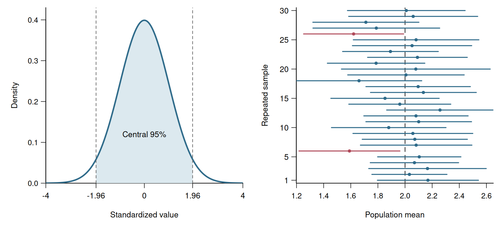
A confidence interval is random because its endpoints depend on the sample.
The population parameter is fixed but unknown.
Thus, about 95% of the intervals constructed from repeated large samples cover the true parameter.
The particular interval calculated from the observed sample either covers the parameter or it does not.
It is therefore incorrect to say that the fixed parameter has a 95% probability of lying in the particular interval we calculated.

Class Size Confidence Interval
We regress test scores on the student-teacher ratio, the percentage of English learners and the percentage eligible for subsidized lunch, including an intercept.
The argument df = Inf selects standard normal critical values:
        2.5 %     97.5 %
STR -1.527656 -0.4689619
The calculation uses \widehat\beta_2\pm1.96\,\mathrm{se}_{HC1}(\widehat\beta_2) =-0.998\pm1.96\cdot0.270.
The approximate 95% HC1 confidence interval is [-1.528,-0.469].
It describes uncertainty about the population mean test-score difference for one more student per teacher in this model.
The comparison is between districts with the same percentages of English learners and students eligible for subsidized lunch.
The probability that the random interval covers the population coefficient approaches 0.95 as n grows.
This is the coverage probability of the confidence interval.
6.7 Confidence Intervals for Effects
Many effects from Section 5 depend on several regression coefficients.
A Quadratic Marginal Effect
We return to the quadratic wage–experience model from Section 5: Y_i=\gamma_1+\gamma_2 A_i+\gamma_3 A_i^2+u_i, \qquad E[u_i\mid A_i]=0.
Here, Y_i is hourly wage and A_i is years of experience.
The marginal effect and its estimator are ME_A(a)=\gamma_2+2a\gamma_3, \qquad \widehat{ME}_A(a)=\widehat\gamma_2+2a\widehat\gamma_3.
The variance rules from Section 3 give \mathrm{Var}\!\left(\widehat{ME}_A(a)\right) =\mathrm{Var}(\widehat\gamma_2) +4a^2\mathrm{Var}(\widehat\gamma_3) +4a\,\mathrm{Cov}(\widehat\gamma_2,\widehat\gamma_3).
Estimate these variances and the covariance using the HC1 covariance matrix. The square root of the result is the effect’s standard error.
The covariance term matters because the coefficient estimates generally move together across samples.
The CEF is quadratic in experience. At a fixed experience level, however, the marginal effect is a linear combination of the coefficients.
Linear Combinations
More generally, let \boldsymbol r be a known, fixed vector of weights and write the effect as \theta=\boldsymbol r'\boldsymbol\beta.
Its estimator and robust standard error are \widehat\theta=\boldsymbol r'\widehat{\boldsymbol\beta}, \qquad \mathrm{se}(\widehat\theta) =\sqrt{ \boldsymbol r' \widehat{\mathrm{Var}}_{HC1} (\widehat{\boldsymbol\beta}) \boldsymbol r }. \tag{6.8}
For \boldsymbol\gamma=(\gamma_1,\gamma_2,\gamma_3)', take \boldsymbol r(a)=(0,1,2a)'.
This gives the same variance formula in compact notation.
Experience at 20 Years
We estimate the model using the CPS sample and store its full HC1 covariance matrix as V.
                (Intercept)  experience I(experience^2)
(Intercept)      0.05345236 -0.00491257    0.0000907417
experience      -0.00491257  0.00061160   -0.0000127614
I(experience^2)  0.00009074 -0.00001276    0.0000002875
The rows and columns correspond to the intercept, experience and squared experience.
Taking square roots of the diagonal entries gives the HC1 standard errors:
The table uses V to report the coefficients and their HC1 standard errors:
modelsummary(quadratic_fit, vcov = V,
gof_map = "nobs", fmt = 4)| (1) | |
|---|---|
| (Intercept) | 14.5198 |
| (0.2312) | |
| experience | 0.9073 |
| (0.0247) | |
| I(experience^2) | -0.0171 |
| (0.0005) | |
| Num.Obs. | 50742 |
At 20 years of experience, the weights are \boldsymbol r(20)=(0,1,40)'. We calculate the effect, its standard error and its 95% interval:
At 20 years of experience, the estimated marginal effect is USD 0.223 in hourly wage per year of experience.
Its HC1 standard error is 0.00712, and its approximate 95% confidence interval is [0.209,0.237].
In this example, the estimated covariance between \widehat\gamma_2 and \widehat\gamma_3 is negative.
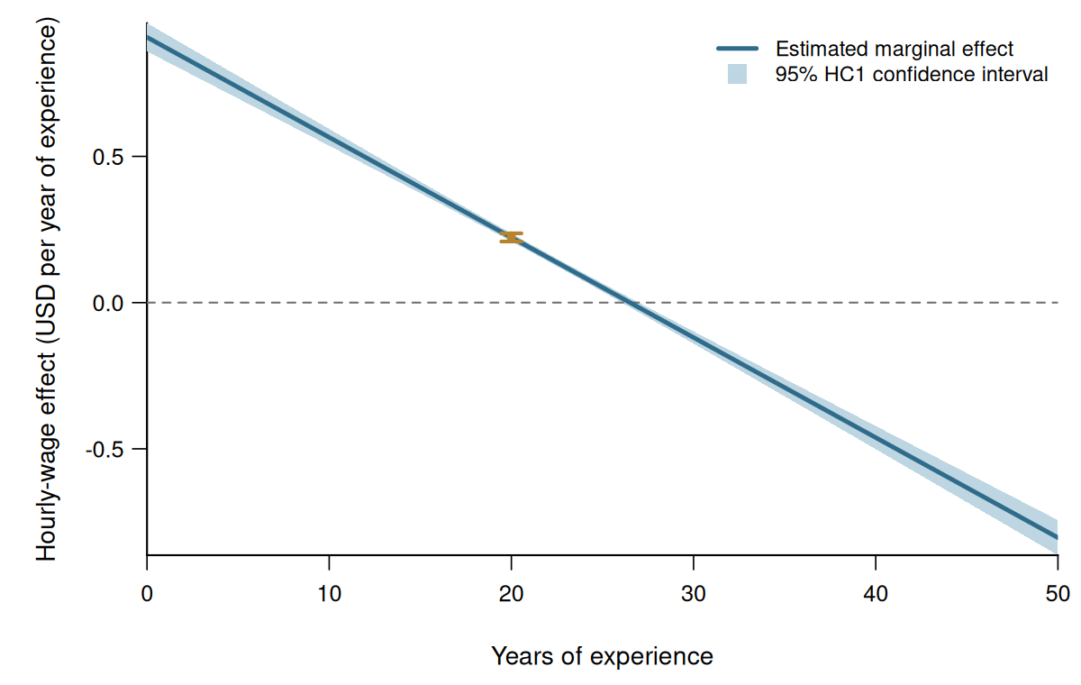
Each vertical slice of the shaded area is a confidence interval at one fixed experience level.
6.8 Leverage and HC3
HC0 uses residuals from the same observations used to estimate the regression.
Some observations pull their fitted values strongly toward their own outcomes. Their residuals are then small compared with the prediction errors obtained when those observations are excluded.
Leverage Values
The hat matrix \boldsymbol H maps observed outcomes into fitted values. Using the OLS formula, \widehat{\boldsymbol Y} =\boldsymbol X\widehat{\boldsymbol\beta} =\boldsymbol X(\boldsymbol X'\boldsymbol X)^{-1} \boldsymbol X'\boldsymbol Y =\boldsymbol H\boldsymbol Y.
Its i-th diagonal entry h_{ii} is the leverage value or hat value of observation i.
Holding all regressors and other outcomes fixed, increasing Y_i by one increases its own fitted value by h_{ii}.
From the hat matrix, h_{ii} =\boldsymbol X_i' (\boldsymbol X'\boldsymbol X)^{-1} \boldsymbol X_i.
The leverage values:
- depend only on the regressors,
- satisfy 0\leq h_{ii}\leq1,
- sum to k and therefore have sample average k/n.
As a rule of thumb, values above 2k/n, twice the average leverage, are considered high and require closer inspection.
In a simple regression with an intercept, h_{ii} = \frac{1}{n} + \frac{(Z_i-\overline Z)^2} {\sum_{\ell=1}^n(Z_\ell-\overline Z)^2}.
Leverage is therefore high when the regressor value lies far from the center of the sample.
In multiple regression, high leverage indicates an unusual combination of regressor values.
A high-leverage observation is not necessarily influential. Its influence also depends on its residual.
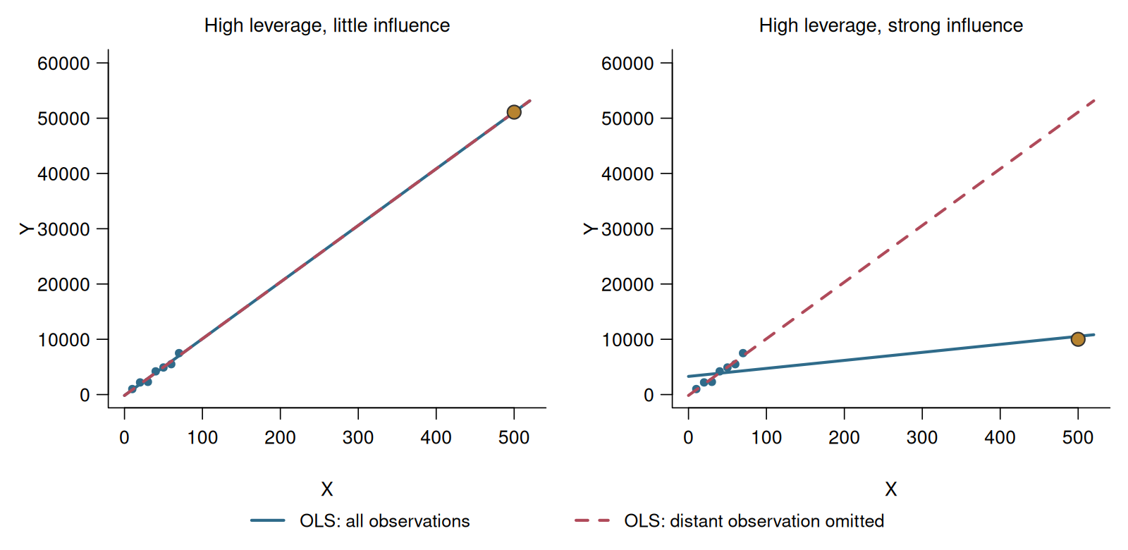
The distant observation has the same leverage, h_{88}=0.987, in both panels.
On the left, removing it leaves the fitted line unchanged. On the right, removing it changes the slope substantially.
High leverage alone is therefore not a reason to delete an observation.
Unusual regressor values are often plausible in economic data. For example, a sample may contain a few individuals with very high incomes alongside many with low incomes.
Inspect high-leverage observations individually to assess whether their regressor values are plausible. Such checks may reveal measurement, coding or data-preparation errors.
Leave-One-Out Residuals
Let \widehat{\boldsymbol\beta}_{(-i)} be the OLS estimator obtained when observation i is omitted. That is, \widehat{\boldsymbol\beta}_{(-i)} satisfies the moment condition \sum_{\substack{\ell=1\\\ell\neq i}}^n \boldsymbol X_\ell \left(Y_\ell-\boldsymbol X_\ell' \widehat{\boldsymbol\beta}_{(-i)}\right) =\boldsymbol0.
The leave-one-out prediction at \boldsymbol X_i is \widehat Y_{i,(-i)} :=\boldsymbol X_i'\widehat{\boldsymbol\beta}_{(-i)}.
The corresponding prediction error is \widehat u_{i,(-i)}:=Y_i-\widehat Y_{i,(-i)}.
Adding observation i to the sum and subtracting the full-sample moment condition gives \begin{aligned} \left(\sum_{\ell=1}^n\boldsymbol X_\ell\boldsymbol X_\ell'\right) \left(\widehat{\boldsymbol\beta} -\widehat{\boldsymbol\beta}_{(-i)}\right) &= \sum_{\ell=1}^n \boldsymbol X_\ell \left(Y_\ell-\boldsymbol X_\ell' \widehat{\boldsymbol\beta}_{(-i)}\right)\\ &=\boldsymbol X_i\widehat u_{i,(-i)}. \end{aligned}
Using \sum_{\ell=1}^n\boldsymbol X_\ell\boldsymbol X_\ell'=n\widehat{\boldsymbol Q}, we obtain \widehat{\boldsymbol\beta} -\widehat{\boldsymbol\beta}_{(-i)} =\frac1n\widehat{\boldsymbol Q}^{-1} \boldsymbol X_i\widehat u_{i,(-i)}. \tag{6.9}
Multiplying by \boldsymbol X_i' gives the change in the fitted value: \widehat Y_i-\widehat Y_{i,(-i)} =\underbrace{\frac1n\boldsymbol X_i' \widehat{\boldsymbol Q}^{-1}\boldsymbol X_i}_{h_{ii}} \widehat u_{i,(-i)}.
Subtract this change from the leave-one-out prediction error: \begin{aligned} \widehat u_i &=(Y_i-\widehat Y_{i,(-i)}) -(\widehat Y_i-\widehat Y_{i,(-i)})\\ &=\widehat u_{i,(-i)}-h_{ii}\widehat u_{i,(-i)}\\ &=(1-h_{ii})\widehat u_{i,(-i)}. \end{aligned}
Thus, the leave-one-out residual is \widehat u_{i,(-i)} = \frac{\widehat u_i}{1-h_{ii}}. \tag{6.10}
The factor 1-h_{ii} shows how leverage reduces the residual’s absolute value relative to the leave-one-out prediction error.
For example, if the leave-one-out error is 4 and h_{ii}=0.25, including observation i moves its fitted value by 1 toward Y_i. The ordinary residual is then 3.
In the right panel of Figure 6.5, compare the distant point’s vertical distances from the two lines.
Its ordinary residual uses the solid full-sample line; its much larger leave-one-out residual uses the dashed line.
HC3 Correction
HC3 keeps the HC0 sandwich structure and replaces each squared ordinary residual by its squared leave-one-out residual: \widehat u_i^2 \quad\longrightarrow\quad \widehat u_{i,(-i)}^2 =\frac{\widehat u_i^2}{(1-h_{ii})^2}.
HC3 Covariance Matrix
Define \widehat{\boldsymbol\Omega}_{HC3} := \frac{1}{n}\sum_{i=1}^n \frac{\widehat u_i^2}{(1-h_{ii})^2} \boldsymbol X_i\boldsymbol X_i'.
The HC3 covariance matrix is \widehat{\mathrm{Var}}_{HC3} (\widehat{\boldsymbol\beta}) := \frac{1}{n} \widehat{\boldsymbol Q}^{-1} \widehat{\boldsymbol\Omega}_{HC3} \widehat{\boldsymbol Q}^{-1}.
When h_{ii} is high, (1-h_{ii})^2 is small. HC3 therefore multiplies the squared OLS residual by a larger adjustment.
HC0, HC1, and HC3 are asymptotically equivalent. Their differences are finite-sample adjustments.
HC1 remains our routine default. HC3 is especially useful in smaller samples or when leverage values are unusually large.
Under zero conditional mean and homoskedasticity, our i.i.d. model gives E[\widehat u_i^2\mid\boldsymbol X] =(1-h_{ii})\sigma^2.
Dividing \widehat u_i^2 by one factor 1-h_{ii} corrects this downward bias. This motivates HC2.
HC3 uses two factors because it squares the leave-one-out residual.
Food Expenditure
The data from Engel’s 1857 study contain annual income and food expenditure for 235 Belgian working-class households. Both variables are measured in Belgian francs.
We use the dataset from the quantreg package, also used by Koenker and Bassett (1982).
We fit a simple linear specification:
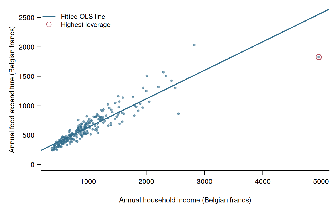
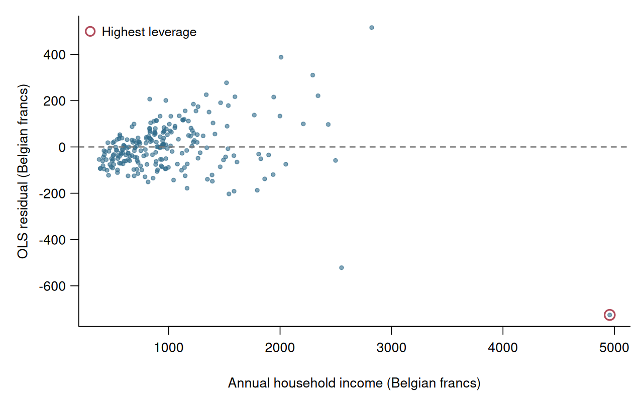
The residuals are more widely spread at higher incomes, suggesting heteroskedasticity.
The table reports the same OLS estimates with three different standard-error estimators. The classical standard errors assume homoskedasticity.
modelsummary(
  list("Classical" = engel_fit,
       "HC1" = engel_fit,
       "HC3" = engel_fit),
  vcov = list("IID", "HC1", "HC3"),
  gof_map = "nobs"
)| Classical | HC1 | HC3 | |
|---|---|---|---|
| (Intercept) | 147.475 | 147.475 | 147.475 |
| (15.957) | (46.648) | (59.955) | |
| income | 0.485 | 0.485 | 0.485 |
| (0.014) | (0.052) | (0.066) | |
| Num.Obs. | 235 | 235 | 235 |
According to the fitted regression, households with one franc more annual income spend, on average, 0.485 francs more on food.
The income coefficient’s standard errors are 0.014, 0.052 and 0.066. Its HC3 standard error is about 28% larger than its HC1 standard error.
We calculate the largest leverage from the fitted model:
The highest leverage is 0.255, compared with the average k/n=2/235=0.009.
For this observation, the residual and squared-residual multipliers are \frac{1}{1-h_{ii}}= 1.34, \qquad \frac{1}{(1-h_{ii})^2}= 1.80.
HC1 multiplies every squared residual by the same factor: \frac{n}{n-k}=\frac{235}{233}= 1.009.
These factors multiply residuals or squared residuals, not the final standard error.
A robust standard error can be smaller or larger than its homoskedastic-only counterpart.
Jackknife
HC3 is also called a jackknife-type robust covariance estimator.
The jackknife removes one observation at a time and measures how much the estimate changes. For coefficient j, \mathrm{se}_{HC3}(\widehat\beta_j)^2 =\sum_{i=1}^n (\widehat\beta_{j,(-i)}-\widehat\beta_j)^2. \tag{6.11}
Thus, HC3 records how sensitive the coefficient estimate is to deleting individual observations.
Combining Equation 6.9 and Equation 6.10 gives \begin{aligned} &\sum_{i=1}^n \left(\widehat{\boldsymbol\beta}_{(-i)}-\widehat{\boldsymbol\beta}\right) \left(\widehat{\boldsymbol\beta}_{(-i)}-\widehat{\boldsymbol\beta}\right)'\\ &\quad=\frac1{n^2}\widehat{\boldsymbol Q}^{-1} \left[\sum_{i=1}^n \boldsymbol X_i\boldsymbol X_i'\widehat u_{i,(-i)}^2\right] \widehat{\boldsymbol Q}^{-1}\\ &\quad=\frac1n\widehat{\boldsymbol Q}^{-1} \widehat{\boldsymbol\Omega}_{HC3}\widehat{\boldsymbol Q}^{-1} =\widehat{\mathrm{Var}}_{HC3}(\widehat{\boldsymbol\beta}). \end{aligned}
The j-th diagonal entry gives Equation 6.11.
6.9 Classical Inference
The preceding confidence intervals use HC1 standard errors and a large-sample normal approximation.
The traditional bachelor-level approach strengthens the assumptions and obtains exact finite-sample inference.
Throughout this subsection, assume n>k and that the regressor matrix \boldsymbol X has full column rank.
Let \boldsymbol u=(u_1,\ldots,u_n)' collect the regression errors.
Conditional Mean
Under i.i.d. sampling, the zero conditional mean condition implies E[\boldsymbol u\mid\boldsymbol X]=\boldsymbol 0.
Conditioning holds the regressor values fixed while considering repeated outcomes.
Using the data-matrix notation from Section 4, \boldsymbol X'\boldsymbol X =\sum_{i=1}^n\boldsymbol X_i\boldsymbol X_i' =n\widehat{\boldsymbol Q}, \qquad \boldsymbol X'\boldsymbol u =\sum_{i=1}^n\boldsymbol X_i u_i.
The OLS decomposition from Section 6.4 can therefore be written as \begin{aligned} \widehat{\boldsymbol\beta} &=\boldsymbol\beta+\widehat{\boldsymbol Q}^{-1} \frac1n\sum_{i=1}^n\boldsymbol X_i u_i\\ &=\boldsymbol\beta +(\boldsymbol X'\boldsymbol X)^{-1}\boldsymbol X'\boldsymbol u. \end{aligned}
Taking the conditional expectation gives \begin{aligned} E[\widehat{\boldsymbol\beta}\mid\boldsymbol X] &=\boldsymbol\beta +(\boldsymbol X'\boldsymbol X)^{-1}\boldsymbol X' E[\boldsymbol u\mid\boldsymbol X]\\ &=\boldsymbol\beta. \end{aligned}
Thus, OLS is conditionally unbiased. At fixed regressor values, the mean of its estimates across repeated outcomes equals the population coefficient vector.
Unbiasedness describes the center of the sampling distribution at a given sample size. Consistency describes concentration around the population parameter as the sample size grows.
Homoskedastic Covariance Matrix
Under homoskedasticity, \mathrm{Var}(\boldsymbol u\mid\boldsymbol X) =\sigma^2\boldsymbol I_n, where \boldsymbol I_n is the n\times n identity matrix.
Applying the covariance rule to the OLS decomposition gives \begin{aligned} \mathrm{Var}(\widehat{\boldsymbol\beta}\mid\boldsymbol X) &=(\boldsymbol X'\boldsymbol X)^{-1}\boldsymbol X' (\sigma^2\boldsymbol I_n)\boldsymbol X (\boldsymbol X'\boldsymbol X)^{-1}\\ &=\sigma^2(\boldsymbol X'\boldsymbol X)^{-1}. \end{aligned}
The same homoskedasticity condition gives \boldsymbol\Omega=\sigma^2\boldsymbol Q in the large-sample formula.
Replacing the unknown error variance by the adjusted residual variance gives the classical covariance matrix estimator: \widehat{\mathrm{Var}}_{hom} (\widehat{\boldsymbol\beta}) =s_{\widehat u}^2 (\boldsymbol X'\boldsymbol X)^{-1}, where s_{\widehat u}^2 =\frac{1}{n-k}\sum_{i=1}^n\widehat u_i^2.
Here, k is the number of estimated coefficients, including the intercept.
The homoskedastic standard error \mathrm{se}_{hom}(\widehat\beta_j) is the square root of diagonal entry j.
Without homoskedasticity, this covariance matrix estimator is generally invalid.
Gaussian Regression Model
Gaussian Regression Model
Conditional on the regressor matrix \boldsymbol X, the errors are independent and normally distributed, with mean zero and the same variance: \boldsymbol u\mid\boldsymbol X \sim\mathcal N(\boldsymbol 0,\sigma^2\boldsymbol I_n).
This assumption concerns the conditional errors and implies that the dependent variable is normally distributed conditional on the regressors. It does not require the regressors to be normally distributed.
Holding \boldsymbol X fixed, the OLS estimator is a linear transformation of \boldsymbol u. Therefore, \widehat{\boldsymbol\beta}\mid\boldsymbol X \sim\mathcal N\!\left( \boldsymbol\beta, \sigma^2(\boldsymbol X'\boldsymbol X)^{-1} \right).
This is an exact conditional distribution for any fixed sample size n. Its covariance depends on \boldsymbol X, so the unconditional distribution may not be normal.
Standardizing each coefficient gives Z_j := \frac{\widehat\beta_j-\beta_j} {\sigma \sqrt{[(\boldsymbol X'\boldsymbol X)^{-1}]_{jj}}} \sim\mathcal N(0,1).
Chi-Squared Distribution
Chi-Squared Distribution
Let Z_1,\ldots,Z_\nu be independent standard normal variables.
Then V=\sum_{\ell=1}^{\nu}Z_\ell^2 \sim\chi_\nu^2.
The parameter \nu is called the degrees of freedom.
The chi-squared distribution takes only nonnegative values.
Under the Gaussian regression model, \frac{\sum_{i=1}^n \widehat u_i^2}{\sigma^2} = \frac{(n-k)s_{\widehat u}^2}{\sigma^2} \sim\chi_{n-k}^2.
The numerator is the sum of squared OLS residuals. Estimating k coefficients leaves n-k degrees of freedom.
Student t-Distribution
Student t-Distribution
Let Z\sim\mathcal N(0,1), \qquad V\sim\chi_\nu^2, and suppose that Z and V are independent.
Then T=\frac{Z}{\sqrt{V/\nu}} \sim t_\nu.
Under the Gaussian regression model, Z_j and (n-k)s_{\widehat u}^2/\sigma^2 are independent. Therefore, \begin{aligned} T_j &:= \frac{\widehat\beta_j-\beta_j} {\mathrm{se}_{hom}(\widehat\beta_j)} = Z_j\frac{\sigma}{s_{\widehat u}}\\ &=\frac{Z_j}{ \sqrt{\dfrac{\sum_{i=1}^n \widehat u_i^2/\sigma^2}{n-k}} } \sim t_{n-k}. \end{aligned}
Replacing the unknown error standard deviation \sigma by s_{\widehat u} therefore changes the reference distribution from standard normal to Student t.
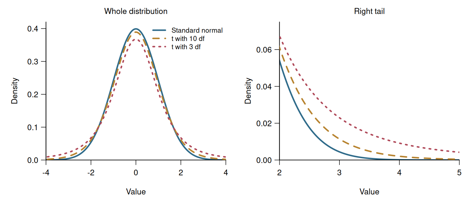
The t_\nu distribution is symmetric and has heavier tails than the standard normal distribution.
Its denominator is random. This additional uncertainty produces the heavier tails.
It approaches \mathcal N(0,1) as \nu increases.
Exact t-Interval
Let t_{\nu,p} denote the p-quantile of the t_\nu distribution.
Exact t-Inference
Suppose the Gaussian regression model holds, n>k, and the regressor matrix has full column rank. Then \frac{\widehat\beta_j-\beta_j} {\mathrm{se}_{hom}(\widehat\beta_j)} \sim t_{n-k}.
Using the homoskedastic standard error gives the exact interval \left[ \widehat\beta_j -t_{n-k,1-\alpha/2}\mathrm{se}_{hom}(\widehat\beta_j), \ \widehat\beta_j +t_{n-k,1-\alpha/2}\mathrm{se}_{hom}(\widehat\beta_j) \right].
Under the Gaussian regression model, the interval has coverage 1-\alpha for any fixed sample size n.
The two approaches can now be compared:
| Main practical route | Classical route |
|---|---|
| Heteroskedasticity allowed | Homoskedasticity required |
| HC1 standard errors | Homoskedastic standard errors |
| Large-sample normal approximation | Exact finite-sample t-distribution |
| No conditional normality required | Conditional normality required |
As the degrees of freedom increase, the t-quantiles approach the standard normal quantiles: t_{n-k,\,1-\alpha/2}\longrightarrow z_{1-\alpha/2} \qquad\text{as }n-k\to\infty.
We can therefore also use t_{n-k}-quantiles with HC-type standard errors. Under our large-sample assumptions, the resulting confidence intervals remain asymptotically valid.
For the same standard error, t-quantiles give wider intervals than normal quantiles. The difference becomes small when n-k is large.
Using t-quantiles with robust standard errors is common in statistical software, although defaults differ. This does not make robust confidence intervals exact in finite samples.