library(AER)
library(modelsummary)
data("CASchools")
CASchools$STR = CASchools$students / CASchools$teachers
CASchools$score = (CASchools$read + CASchools$math) / 2

simple_class_size_fit = lm(score ~ STR, data = CASchools)
class_size_fit = lm(score ~ STR + english + lunch, data = CASchools)
expenditure_fit = lm(score ~ STR + english + lunch + expenditure,
                     data = CASchools)
class_size_models = list("(1)" = simple_class_size_fit,
                         "(2)" = class_size_fit,
"(3)" = expenditure_fit)7 Testing
Section 6 used point estimates, standard errors, and critical values to construct confidence intervals.
Hypothesis tests evaluate claims about a population using a test statistic and its distribution under the claim being tested.
We first introduce the general testing framework, then apply it to regression coefficients and model diagnostics.
7.1 Statistical Hypotheses
A statistical hypothesis is a statement about the population distribution. It is often expressed as a restriction on one or more population parameters.
Null and Alternative Hypotheses
The null hypothesis H_0 is the claim being tested.
The alternative hypothesis H_1 describes the departures from H_0 that the test is designed to detect.
For example, let \theta be a scalar population parameter and \theta_0 a hypothesized value. A two-sided test considers H_0:\theta=\theta_0 \qquad\text{against}\qquad H_1:\theta\neq\theta_0. \tag{7.1}
Here, \theta may be a population mean, a regression coefficient or a marginal effect.
Other hypotheses restrict several parameters jointly or specify a property of the population distribution, such as homoskedasticity or normality.
Test Decisions
A test statistic is a function of the sample used to assess disagreement with H_0. Write S for a general test statistic.
Its null distribution describes the values it would take across repeated samples if H_0 were true.
A rejection region \mathcal R_\alpha contains values that are unlikely under H_0: \begin{aligned} \text{reject }H_0 &\quad\text{if }S\in\mathcal R_\alpha,\\ \text{fail to reject }H_0 &\quad\text{if }S\notin\mathcal R_\alpha. \end{aligned}
We choose the significance level \alpha before examining the test result. Common choices are 0.10, 0.05 and 0.01.
A level-\alpha test satisfies P(\text{reject }H_0\mid H_0\text{ is true}) \leq\alpha.
An asymptotic level-\alpha tests satisfies \lim_{n\to\infty} P(\text{reject }H_0\mid H_0\text{ is true}) \leq \alpha.
Rejecting H_0 provides evidence against it at the chosen significance level.
Failing to reject H_0 means that the sample is compatible with it at that level.
Either decision can be incorrect. We therefore assess a test through the probabilities of rejecting a true null hypothesis and failing to reject a false one.
Testing Errors and Power
| Population situation | Fail to reject H_0 | Reject H_0 |
|---|---|---|
| H_0 is true | Correct decision | Type I error |
| H_0 is false | Type II error | Correct decision |
The significance level controls the Type I error probability.
The power at a particular alternative is the probability of rejecting H_0 when that alternative is true.
At that alternative, \mathrm{Power}=1-P(\text{Type II error}).
Larger samples and larger departures from the null generally increase power.
For the asymptotic tests considered here, the Type I error probability approaches \alpha as n increases.
A test is called consistent if, against each fixed alternative, its Type II error probability approaches zero and its power approaches one.
7.2 Testing One Restriction
Let \widehat\theta estimate a population parameter \theta, and let \mathrm{se}(\widehat\theta) be a valid standard error.
Suppose the estimator and standard error satisfy \frac{\widehat\theta-\theta}{\mathrm{se}(\widehat\theta)} \overset d\to\mathcal N(0,1). \tag{7.2}
Recall that this holds for the sample mean and regression coefficients under suitable conditions.
t-Statistic and Two-Sided Test
For H_0: \theta = \theta_0, define the standardized distance T :=\frac{\widehat\theta-\theta_0} {\mathrm{se}(\widehat\theta)}. \tag{7.3}
Under H_0, the standardized normal limit in Equation 7.2 gives T\overset{d}{\to}\mathcal N(0,1).
We reject H_0 at significance level \alpha if |T|>z_{1-\alpha/2}. \tag{7.4}
Recall that, for Z\sim\mathcal N(0,1), \begin{aligned} P(|Z|>z_{1-\alpha/2}) &=1-P(-z_{1-\alpha/2}\leq Z\leq z_{1-\alpha/2})\\ &=\alpha. \end{aligned}
Under H_0, the standardized normal limit therefore implies P(|T|>z_{1-\alpha/2})\longrightarrow\alpha \qquad\text{as }n\to\infty.
Thus, the test has asymptotic level \alpha.
The statistic is often called a t-statistic. Here, its reference distribution is the standard normal distribution implied by the limit above.
The name does not imply an exact Student t distribution. Such a result requires additional assumptions.
Large positive and negative values provide evidence against the two-sided null. For a 5% test, the critical values are -1.96 and 1.96.
A Population Mean
For an i.i.d. sample with mean \mu and finite positive variance, Sections 6.1 and 6.3 give the standard error and CLT for \overline Y_n.
To test H_0:\mu=\mu_0, set \widehat\theta=\overline Y_n and use the sample standard deviation \widehat\sigma_Y from Section 6.1: T=\frac{\overline Y_n-\mu_0} {\widehat\sigma_Y/\sqrt n} \overset d\to\mathcal N(0,1) \qquad\text{under }H_0.
The observations themselves need not be normally distributed for this large-sample test.
Sample Size and Power
To illustrate power, suppose the population standard deviation \sigma_Y is known. Using it in the denominator gives the normal approximation T=\frac{\overline Y_n-\mu_0}{\sigma_Y/\sqrt n} \overset{\mathrm{approx.}}{\sim} \mathcal N\!\left(\frac{\sqrt n(\mu-\mu_0)}{\sigma_Y},\,1\right).
Under H_0, the distribution is centered at zero. Under a fixed alternative \mu\neq\mu_0, increasing n moves its center farther from zero.
Consider H_0:\mu=100 when the population mean is actually 102 and \sigma_Y=10. Both panels use the same 5% rejection rule, |T|>1.96.
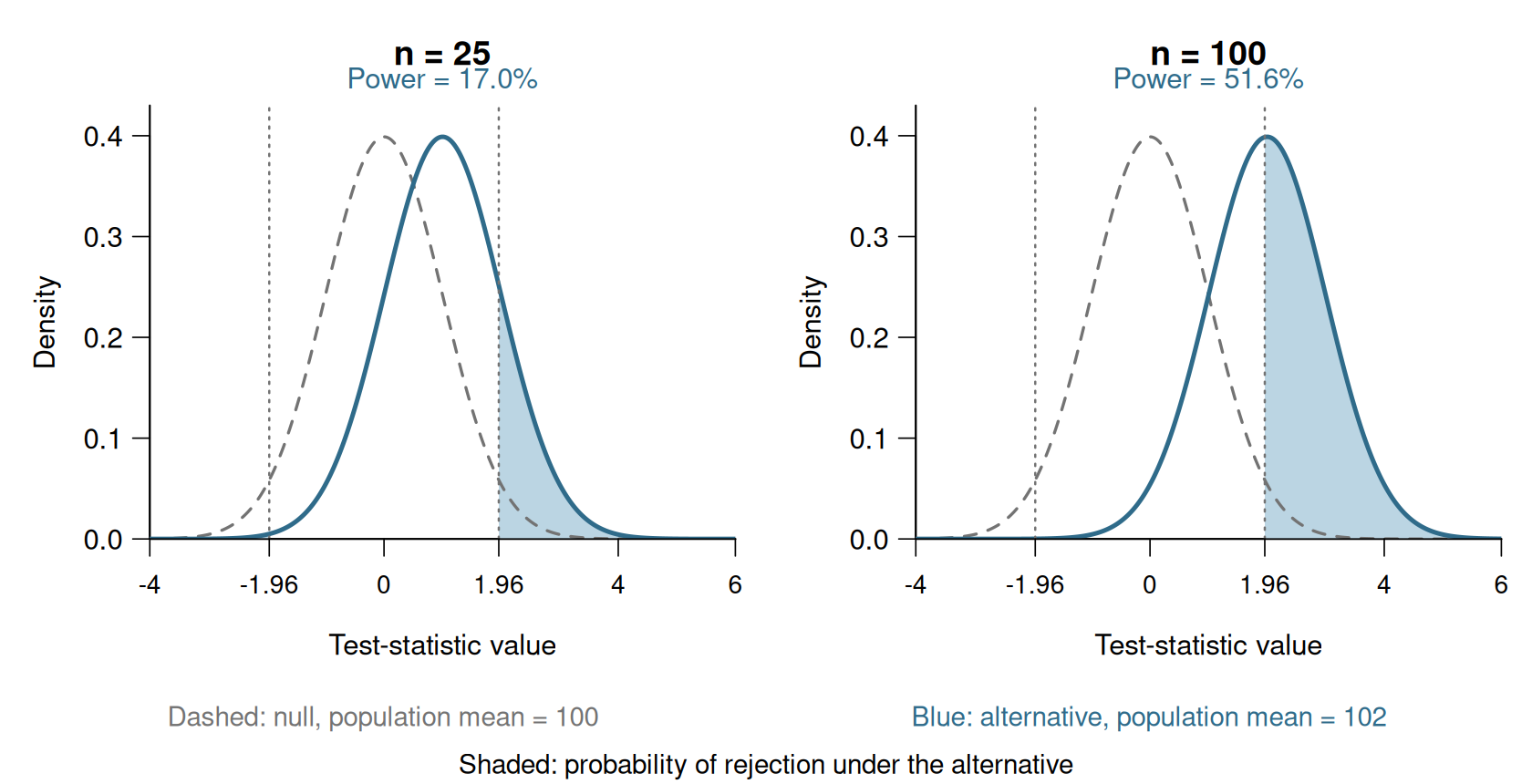
Power increases from 17.0\% at n=25 to 51.6\% at n=100. With the smaller sample, the test usually fails to reject even though the null is false.
The larger sample estimates the mean more precisely, making the same population difference easier to detect.
Regression Coefficients
We now apply the same test to OLS coefficients. Recall the regression model Y_i=\boldsymbol X_i'\boldsymbol\beta+u_i, \qquad E[u_i\mid\boldsymbol X_i]=0.
As in Section 6, assume i.i.d. observations, finite entries of \boldsymbol Q and \boldsymbol\Omega, and invertible \boldsymbol Q. For the coefficient being tested, assume a positive asymptotic variance.
To test H_0:\beta_j=\beta_{j,0}, set \theta=\beta_j and \widehat\theta=\widehat\beta_j: T=\frac{\widehat\beta_j-\beta_{j,0}} {\mathrm{se}(\widehat\beta_j)} \overset d\to\mathcal N(0,1) \qquad\text{under }H_0\text{ as }n\to\infty.
Section 6 establishes the standardized normal limit for these coefficients. HC1 or HC3 provides a suitable standard error under the maintained conditions.
Here, \mathrm{se} denotes a valid standard error.
As in Section 6.6, \mathrm{se}(\widehat\beta_j)/\mathrm{sd}(\widehat\beta_j)\overset p\to1, where \mathrm{sd}(\widehat\beta_j) denotes the standard deviation in the large-sample normal approximation.
Class Size Example
We compare the three class-size specifications from Section 5. Model (2) is the controlled regression used for inference in Section 6: \mathrm{score}_i =\beta_1+\beta_2\mathrm{STR}_i +\beta_3\mathrm{english}_i +\beta_4\mathrm{lunch}_i+u_i.
The table reports all coefficients, with HC1 standard errors in parentheses:
modelsummary(class_size_models, vcov = "HC1", gof_map = "nobs")| (1) | (2) | (3) | |
|---|---|---|---|
| (Intercept) | 698.933 | 700.150 | 665.988 |
| (10.364) | (5.568) | (10.377) | |
| STR | -2.280 | -0.998 | -0.235 |
| (0.519) | (0.270) | (0.325) | |
| english | -0.122 | -0.128 | |
| (0.033) | (0.032) | ||
| lunch | -0.547 | -0.546 | |
| (0.024) | (0.023) | ||
| expenditure | 0.004 | ||
| (0.001) | |||
| Num.Obs. | 420 | 420 | 420 |
For Model (2), consider the hypothesis that the population coefficient on the student-teacher ratio is zero: H_0:\beta_2=0 \qquad\text{against}\qquad H_1:\beta_2\neq0.
The estimate and its HC1 standard error are -0.998 and 0.270.
Therefore, T=\frac{-0.998-0}{0.270}=-3.696.
Because |T|>1.96, we reject H_0 at the 5% level.
According to the fitted model, districts with one more student per teacher and the same percentages of English learners and students eligible for subsidized lunch have, on average, test scores 0.998 points lower.
The test provides evidence that this population coefficient differs from zero.
For Model (3), we also test whether its STR coefficient is zero. Here, T=\frac{-0.2354-0}{0.3248}=-0.725.
Because |T|<1.96, we fail to reject at the 5% level.
Model (3) compares districts with the same expenditure per pupil, as well as the same English-learner and subsidized-lunch percentages.
In the mediator story from Section 5.4, holding expenditure fixed excludes part of the effect of hiring more teachers. The two tests therefore concern different conditional comparisons.
7.3 p-Values
Unless stated otherwise, we calculate p-values using the limiting null distribution of the test statistic.
p-Value
For the tests considered here, larger absolute values of the test statistic indicate stronger disagreement with H_0.
Let S_{\mathrm{obs}} be its observed value and let S_0 follow its null reference distribution.
The p-value is p:=P\bigl(|S_0|\geq|S_{\mathrm{obs}}|\bigr).
It is the probability assigned by the null reference distribution to a statistic at least as extreme as the observed one.
Using the limiting null distribution gives a large-sample p-value. Using an exact null distribution gives an exact p-value.
For a two-sided t-test, both large positive and large negative values of T count as evidence against H_0.
The Wald and diagnostic statistics introduced below are nonnegative, so their absolute values equal the statistics themselves.
Using the same reference distribution, the decision rule is \begin{aligned} \text{reject }H_0 &\quad\text{if }p<\alpha,\\ \text{fail to reject }H_0 &\quad\text{if }p\geq\alpha. \end{aligned}
Two-Sided Test of a Scalar Parameter
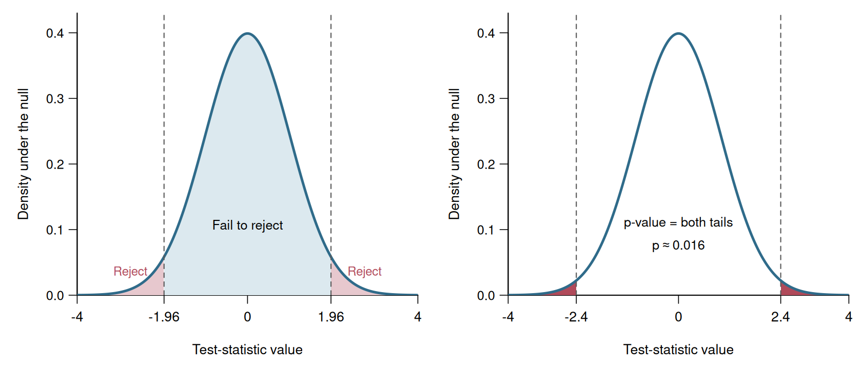
For the large-sample test in Section 7.2, let T_{\mathrm{obs}} be the observed standardized statistic. Its limiting null reference is Z\sim\mathcal N(0,1). Using symmetry, \begin{aligned} p &=P\bigl(|Z|\geq|T_{\mathrm{obs}}|\bigr)\\ &=P(Z\leq-|T_{\mathrm{obs}}|)+P(Z\geq|T_{\mathrm{obs}}|)\\ &=\Phi(-|T_{\mathrm{obs}}|)+1-\Phi(|T_{\mathrm{obs}}|)\\ &=2\left[1-\Phi(|T_{\mathrm{obs}}|)\right]. \end{aligned} \tag{7.5}
This formula applies whenever the standardized estimator has the normal limit in Section 7.2, including the population-mean and regression-coefficient examples.
Class Size Example
For the class-size coefficient in Model (2), insert T_{\mathrm{obs}}=(\widehat\beta_2-0)/\mathrm{se}(\widehat\beta_2)=-3.696: p=2\left[1-\Phi(3.696)\right] =0.0002.
Interpreting a p-Value
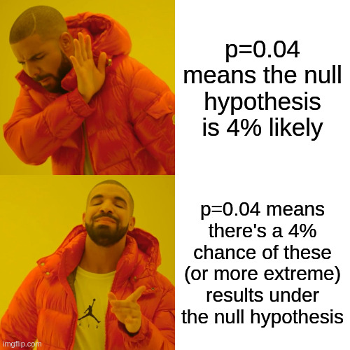
The p-value is calculated under the assumption that H_0 is true.
It is not the probability that H_0 is true.
For example, a p-value of 0.04 means that the reference distribution assigns 4% probability to test statistics at least as extreme as the observed one.
Relation to Confidence Intervals
For the two-sided scalar test in Section 7.2, construct the corresponding confidence interval using the same standard error and critical value.
Then p<\alpha \quad\Longleftrightarrow\quad \theta_0\notin I_{1-\alpha}. \tag{7.6}
For Model (2), we regress test scores on STR, the percentage of English learners and the percentage eligible for subsidized lunch, including an intercept.
The table repeats the coefficient estimates, with HC1 standard errors in parentheses:
modelsummary(list("(2)" = class_size_fit),
vcov = "HC1", fmt = 4, gof_map = "nobs")| (2) | |
|---|---|
| (Intercept) | 700.1500 |
| (5.5685) | |
| STR | -0.9983 |
| (0.2701) | |
| english | -0.1216 |
| (0.0328) | |
| lunch | -0.5473 |
| (0.0241) | |
| Num.Obs. | 420 |
Its 95% HC1 interval for the STR coefficient from Section 6 is [-1.528,-0.469].
It excludes zero but contains -1.
For H_0:\beta_2=-1, the standardized distance is T=\frac{\widehat\beta_2-(-1)}{\mathrm{se}(\widehat\beta_2)} =\frac{-0.9983-(-1)}{0.2701}=0.0063.
Using the fitted estimate and standard error in R:
| Hypothesis | T | p-value | Decision at 5% |
|---|---|---|---|
| H_0:\beta_2=0 | -3.696 | 0.0002 | Reject H_0 |
| H_0:\beta_2=-1 | 0.006 | 0.995 | Fail to reject H_0 |
Thus, a hypothesis test need not concern a zero coefficient.
Failing to reject \beta_2=-1 means that this value is compatible with the data at the chosen level. It does not establish that the coefficient equals -1.
7.4 Statistical Significance
A result is statistically significant at level \alpha when the corresponding null hypothesis is rejected at that level.
Our regression tables use the following stars for tests of H_0:\beta_j=0:
| Stars | p-value |
|---|---|
*** |
p<0.01 |
** |
0.01\leq p<0.05 |
* |
0.05\leq p<0.10 |
Stars provide a compact summary of p-values.
Conventions differ. The default stars in R output use different cutoffs, so always read the table’s legend.
Class Size and Expenditure
We return to the three specifications from Section 5.4. The table now includes significance stars and HC1 standard errors:
modelsummary(
  class_size_models, vcov = "HC1",
  stars = c("*" = 0.10, "**" = 0.05, "***" = 0.01),
  gof_map = "nobs"
)| (1) | (2) | (3) | |
|---|---|---|---|
| * p < 0.1, ** p < 0.05, *** p < 0.01 | |||
| (Intercept) | 698.933*** | 700.150*** | 665.988*** |
| (10.364) | (5.568) | (10.377) | |
| STR | -2.280*** | -0.998*** | -0.235 |
| (0.519) | (0.270) | (0.325) | |
| english | -0.122*** | -0.128*** | |
| (0.033) | (0.032) | ||
| lunch | -0.547*** | -0.546*** | |
| (0.024) | (0.023) | ||
| expenditure | 0.004*** | ||
| (0.001) | |||
| Num.Obs. | 420 | 420 | 420 |
As discussed in Section 6.9, the software uses a t reference distribution with robust standard errors. The resulting tests are large-sample approximations.
- In Models (1) and (2), the STR coefficient is negative and significant at the 1% level.
- In Model (3), its estimate is -0.235, with standard error 0.325 and p-value 0.469. It is not significant at the conventional levels.
The coeftest output displays the test statistics and p-values directly:
t test of coefficients:

               Estimate  Std. Error t value Pr(>|t|)
(Intercept) 665.9881983  10.3768351  64.180 < 0.0001 ***
STR          -0.2353882   0.3248149  -0.725 0.469054
english      -0.1283417   0.0324397  -3.956 < 0.0001 ***
lunch        -0.5463928   0.0231685 -23.583 < 0.0001 ***
expenditure   0.0036220   0.0009447   3.834 0.000146 ***
---
Signif. codes:  0 '***' 0.001 '**' 0.01 '*' 0.05 '.' 0.1 ' ' 1
Adding expenditure changes the comparison: Model (3) holds expenditure per pupil fixed, alongside English learners and subsidized-lunch eligibility.
In the mediator story from Section 5.4, hiring more teachers lowers STR and raises expenditure. Holding expenditure fixed excludes this channel of the policy’s effect.
The insignificant STR coefficient in Model (3) therefore does not establish that a class-size policy has no total effect. The significance stars cannot decide whether expenditure is an appropriate control.
Interpreting Significance
Statistical significance does not measure the size or practical importance of an effect. With a large sample, even a small coefficient may be precisely estimated.
To assess practical importance, report the estimated effect together with a suitable confidence interval.
The effect size describes the magnitude of the relationship. The interval shows the uncertainty around that estimate.
7.5 Testing Several Restrictions
We now apply the testing framework to restrictions on regression coefficients. An effect may depend on several coefficients.
We first distinguish one restriction involving several coefficients from several restrictions tested jointly.
Class Size Slopes for Two Groups
Let \mathrm{HiEL}_i equal one for districts with at least 10% English learners and zero otherwise.
Consider the interaction model \mathrm{score}_i =\beta_1+\beta_2\mathrm{STR}_i+\beta_3\mathrm{HiEL}_i +\beta_4\mathrm{STR}_i\mathrm{HiEL}_i+u_i.
CASchools$HiEL = as.numeric(CASchools$english >= 10)
group_fit = lm(score ~ STR * HiEL, data = CASchools)
V_group = vcovHC(group_fit, type = "HC1")
As in Section 5.7, the class-size slopes are ME_{\mathrm{STR}}(0)=\beta_2, \qquad ME_{\mathrm{STR}}(1)=\beta_2+\beta_4.
Each slope compares districts within the same English-learner group. Their exact percentages of English learners need not be equal.
The table reports HC1 standard errors in parentheses. Its significance stars use the standard normal reference distribution.
group_test = coeftest(
  group_fit, vcov. = V_group, df = Inf
)
modelsummary(
  list("Interaction model" = group_test),
  stars = c("*" = 0.10, "**" = 0.05, "***" = 0.01),
  gof_map = "nobs"
)| Interaction model | |
|---|---|
| * p < 0.1, ** p < 0.05, *** p < 0.01 | |
| (Intercept) | 682.246*** |
| (11.868) | |
| STR | -0.968 |
| (0.589) | |
| HiEL | 5.639 |
| (19.515) | |
| STR × HiEL | -1.277 |
| (0.967) | |
| Num.Obs. | 420 |
One Restriction on Two Coefficients
For the high-English-learner group, consider H_0:\beta_2+\beta_4=0 \qquad\text{against}\qquad H_1:\beta_2+\beta_4\neq0.
This is one restriction on the effect \theta=\beta_2+\beta_4.
Its estimate is \widehat\theta=-0.968-1.277=-2.245. Section 6.7 gives its estimated variance: \begin{aligned} \mathrm{se}(\widehat\theta)^2 &=\widehat{\mathrm{Var}}(\widehat\beta_2) +\widehat{\mathrm{Var}}(\widehat\beta_4)\\ &\quad+2\widehat{\mathrm{Cov}} (\widehat\beta_2,\widehat\beta_4). \end{aligned}
As in Section 6.7, the weights \boldsymbol r=(0,1,0,1)' select \beta_2+\beta_4:
         [,1]
[1,] -2.92807 [,1]
[1,] 0.003410735The standard error is 0.767, so T=\frac{-2.245}{0.767}=-2.928, \qquad p=0.0034.
We reject at the 1% level. According to the fitted model, districts in this group with one more student per teacher have, on average, test scores 2.245 points lower.
The standard error of this effect cannot be read from either coefficient’s standard error alone.
Joint Restrictions
Having no class-size association in either group requires \beta_2=0, \qquad \beta_2+\beta_4=0.
Equivalently, the joint hypotheses are \begin{aligned} H_0:&\quad \beta_2=0\ \text{and}\ \beta_4=0,\\ H_1:&\quad \text{at least one of these restrictions is false}. \end{aligned}
Neither \widehat\beta_2 nor \widehat\beta_4 is individually significant at the 5% level. A joint test nevertheless needs to account for their covariance.
With \boldsymbol\beta=(\beta_1,\beta_2,\beta_3,\beta_4)', write \boldsymbol R =\begin{pmatrix} 0&1&0&0\\ 0&0&0&1 \end{pmatrix}, \qquad \boldsymbol r =\begin{pmatrix}0\\0\end{pmatrix}.
Then \boldsymbol R\boldsymbol\beta=(\beta_2,\beta_4)', and H_0 is \boldsymbol R\boldsymbol\beta=\boldsymbol r.
More generally, linear hypotheses about the regression coefficients take the form H_0:\boldsymbol R\boldsymbol\beta=\boldsymbol r \qquad\text{against}\qquad H_1:\boldsymbol R\boldsymbol\beta\neq\boldsymbol r, \tag{7.7} where
- \boldsymbol R is a q\times k restriction matrix with rank q,
- \boldsymbol r is a q\times1 vector of hypothesized values,
- and q is the number of restrictions.
Full row rank means that no restriction repeats or follows from the others. The values in \boldsymbol r need not be zero.
Wald Test
The estimated distance from the restrictions is \widehat{\boldsymbol d} :=\boldsymbol R\widehat{\boldsymbol\beta}-\boldsymbol r.
Recall the limiting covariance matrix from Section 6.4: \boldsymbol\Sigma_\beta =\boldsymbol Q^{-1}\boldsymbol\Omega\boldsymbol Q^{-1}, \qquad \boldsymbol Q=E[\boldsymbol X_i\boldsymbol X_i'], \boldsymbol\Omega=E[u_i^2\boldsymbol X_i\boldsymbol X_i'].
Let \widehat{\boldsymbol V}=\widehat{\mathrm{Var}}(\widehat{\boldsymbol\beta}) estimate the approximate covariance \boldsymbol\Sigma_\beta/n. The covariance rule from Section 3 gives \widehat{\boldsymbol V}_d :=\widehat{\mathrm{Var}}(\widehat{\boldsymbol d}) =\boldsymbol R\widehat{\boldsymbol V}\boldsymbol R'.
Wald Test for Regression Coefficients
The Wald statistic is W:=\widehat{\boldsymbol d}' \widehat{\boldsymbol V}_d^{-1} \widehat{\boldsymbol d}. \tag{7.8}
Suppose the OLS asymptotic-normality and covariance-estimation conditions from Section 6 hold, and \boldsymbol R\boldsymbol\Sigma_\beta\boldsymbol R' is invertible.
Under H_0, W\overset{d}{\to}\chi_q^2.
We reject at significance level \alpha if W>\chi^2_{q,1-\alpha}.
Here, \chi^2_{q,1-\alpha} is the (1-\alpha)-quantile of the \chi_q^2 distribution.
The large-sample p-value uses the upper tail of the null reference distribution: p=1-F_{\chi_q^2}(W_{\mathrm{obs}}).
The chi-squared distribution from Section 6 takes only nonnegative values. Large values of W indicate a large distance from the null after accounting for sampling uncertainty.
For one restriction using the same covariance estimator, W=T^2.
Thus, the Wald test generalizes the two-sided test to several restrictions.
NoteWhy a chi-squared distribution?
Under the null, the estimated restrictions are jointly asymptotically normal and centered at zero.
Standardizing them jointly accounts for their variances and covariances. The Wald statistic is the sum of squares of these standardized components.
Their limiting distribution consists of q independent standard normal variables. The sum of their squares has the \chi_q^2 distribution.
For the class-size example, we calculate
linearHypothesis(
  group_fit,
  c("STR = 0", "STR:HiEL = 0"),
  vcov. = V_group,
  test = "Chisq"
)
Linear hypothesis test:
STR = 0
STR:HiEL = 0

Model 1: restricted model
Model 2: score ~ STR * HiEL

Note: Coefficient covariance matrix supplied.

  Res.Df Df  Chisq Pr(>Chisq)
1    418
2    416  2 11.276    0.00356 **
---
Signif. codes:  0 '***' 0.001 '**' 0.01 '*' 0.05 '.' 0.1 ' ' 1
The Wald statistic is 11.276. With q=2 restrictions, \chi^2_{2,0.99}=9.210, \qquad p=0.0036.
The same p-value comes from the chi-squared upper tail:
pchisq(11.276, df = 2, lower.tail = FALSE)[1] 0.003559981The four tests answer different questions:
| Question | Null hypothesis | p-value | Decision at 5% |
|---|---|---|---|
| Low-English-learner group’s slope zero? | \beta_2=0 | 0.1002 | Fail to reject |
| High-English-learner group’s slope zero? | \beta_2+\beta_4=0 | 0.0034 | Reject |
| Both slopes equal? | \beta_4=0 | 0.1867 | Fail to reject |
| Both slopes zero? | \beta_2=\beta_4=0 | 0.0036 | Reject |
To understand these results, consider the approximate 95% confidence intervals calculated using HC1 standard errors:
| Population quantity | Estimate | 95% confidence interval |
|---|---|---|
| Low-English-learner group’s slope, \beta_2 | -0.968 | [-2.12,\,0.19] |
| High-English-learner group’s slope, \beta_2+\beta_4 | -2.245 | [-3.75,\,-0.74] |
| Difference between slopes, \beta_4 | -1.277 | [-3.17,\,0.62] |
The first interval includes zero, but also substantial negative slopes. Failing to reject \beta_2=0 therefore does not establish that this group has no class-size association.
For example, a slope of -1.5 lies within both group-specific intervals.
Whether the slopes differ is assessed directly through \beta_4. Its interval includes zero, so there is insufficient evidence of a difference. This does not establish that the slopes are equal.
The joint test provides evidence against both slopes being zero. This is compatible with both slopes being negative and similar in magnitude.
A significant slope in one group and an insignificant slope in the other do not establish a difference between the groups.
Classical t and F Tests
Under the homoskedastic Gaussian regression model from Section 6, the homoskedastic standard error gives an exact null distribution: T_{hom}\sim t_{n-k}.
For example, the exact two-sided p-value is 2[1-F_{t_{n-k}}(|T_{hom,\mathrm{obs}}|)].
The corresponding exact test for several restrictions uses the F distribution.
F Distribution
If A\sim\chi_q^2 and B\sim\chi_\nu^2 are independent, then \frac{A/q}{B/\nu}\sim F_{q,\nu}.
Here, F_{q,\nu} denotes the F distribution with q numerator and \nu denominator degrees of freedom.
Let W_{hom} be the Wald statistic calculated with the homoskedastic covariance estimator. \widehat{\boldsymbol V}_{hom} =s_{\widehat u}^2(\boldsymbol X'\boldsymbol X)^{-1}, \qquad s_{\widehat u}^2=\frac{1}{n-k}\sum_{i=1}^n\widehat u_i^2.
Under the Gaussian model and H_0, F:=\frac{W_{hom}}q\sim F_{q,n-k}.
We reject if F>F_{q,n-k,1-\alpha}, the (1-\alpha)-quantile of this distribution.
For one restriction, F=T_{hom}^2, so the F test and the two-sided t test agree.
For fixed q, let F_\nu\sim F_{q,\nu}. As the denominator degrees of freedom increase, qF_\nu\overset d\longrightarrow\chi_q^2 \qquad\text{as }\nu\to\infty. This connects the classical F test to the large-sample Wald test.
Software also uses t and F reference distributions with robust covariance estimators. Under heteroskedasticity, these give large-sample approximations, not exact finite-sample tests.
7.6 Regression Diagnostics
We assess the fitted model using goodness-of-fit measures, visual diagnostics and formal tests.
We first summarize how well the regression fits the observed data. We then examine residual patterns and test assumptions about the error distribution.
Goodness of Fit and R^2
R-squared
For a regression with an intercept and an outcome that varies in the sample, R^2 :=1- \frac{\sum_{i=1}^n\widehat u_i^2} {\sum_{i=1}^n(Y_i-\overline Y)^2}. \tag{7.9}
It measures the share of the observed sample variation in Y_i accounted for by the fitted regression.
Under these conditions, 0\leq R^2\leq1. The higher the R-squared, the better the OLS regression fits the observed data.
Starting from Model (1), we add English learners in a new Model (4), then subsidized-lunch eligibility to obtain Model (2). All three regressions use the same 420 districts.
english_fit = lm(score ~ STR + english, data = CASchools)
fit_models = list(
  "(1)" = simple_class_size_fit,
  "(4)" = english_fit,
  "(2)" = class_size_fit
)
modelsummary(
  fit_models, vcov = "HC1",
  stars = c("*" = 0.10, "**" = 0.05, "***" = 0.01),
  gof_map = c("nobs", "r.squared")
)| (1) | (4) | (2) | |
|---|---|---|---|
| * p < 0.1, ** p < 0.05, *** p < 0.01 | |||
| (Intercept) | 698.933*** | 686.032*** | 700.150*** |
| (10.364) | (8.728) | (5.568) | |
| STR | -2.280*** | -1.101** | -0.998*** |
| (0.519) | (0.433) | (0.270) | |
| english | -0.650*** | -0.122*** | |
| (0.031) | (0.033) | ||
| lunch | -0.547*** | ||
| (0.024) | |||
| Num.Obs. | 420 | 420 | 420 |
| R2 | 0.051 | 0.426 | 0.775 |
The R^2 values increase from 0.051 to 0.426 and 0.775. Each additional control substantially improves the sample fit in this example.
More generally, adding regressors cannot reduce the ordinary R^2 when the outcome and estimation sample remain unchanged. OLS could always assign zero to the additional coefficients and retain the previous fit.
This property holds even when an added coefficient is statistically insignificant. An increase in R^2 is therefore not a test of significance.
A high R^2 does not establish a correct CEF or a causal relationship.
A very flexible model can also fit random variation in the sample rather than the population relationship. This is overfitting: a close sample fit may come with poor predictions for new observations.
For example, if k=n and \boldsymbol X has full rank, OLS fits every observed outcome exactly and gives R^2=1. This holds regardless of whether the specification describes the population CEF.
A low R^2 does not by itself imply that an estimated conditional-mean effect is uninformative.
Control variables should therefore not be selected by maximizing R^2.
Residual Plots
Section 4.6 compared residuals from a straight-line and a quadratic fit in a generated example.
The fitted value \widehat Y_i=\boldsymbol X_i'\widehat{\boldsymbol\beta} combines the regressors into a single prediction.
A residual-versus-fitted plot compares OLS residuals with fitted values to look for conditional-mean patterns that the model has missed.
A plot against one particular regressor instead focuses on patterns across that variable’s values.
- Systematic changes in average residuals across ranges of the horizontal axis suggest a missed conditional-mean pattern.
- A changing vertical spread suggests that the conditional variance is not constant, as illustrated in Section 6.5.
Changing spread alone does not imply that the conditional mean is misspecified. Conversely, an apparently flat pattern does not establish correct specification.
The diagnostic plots use Model (2), which includes STR, English learners and subsidized-lunch eligibility.
In R, the residual-versus-fitted plot can be drawn with:
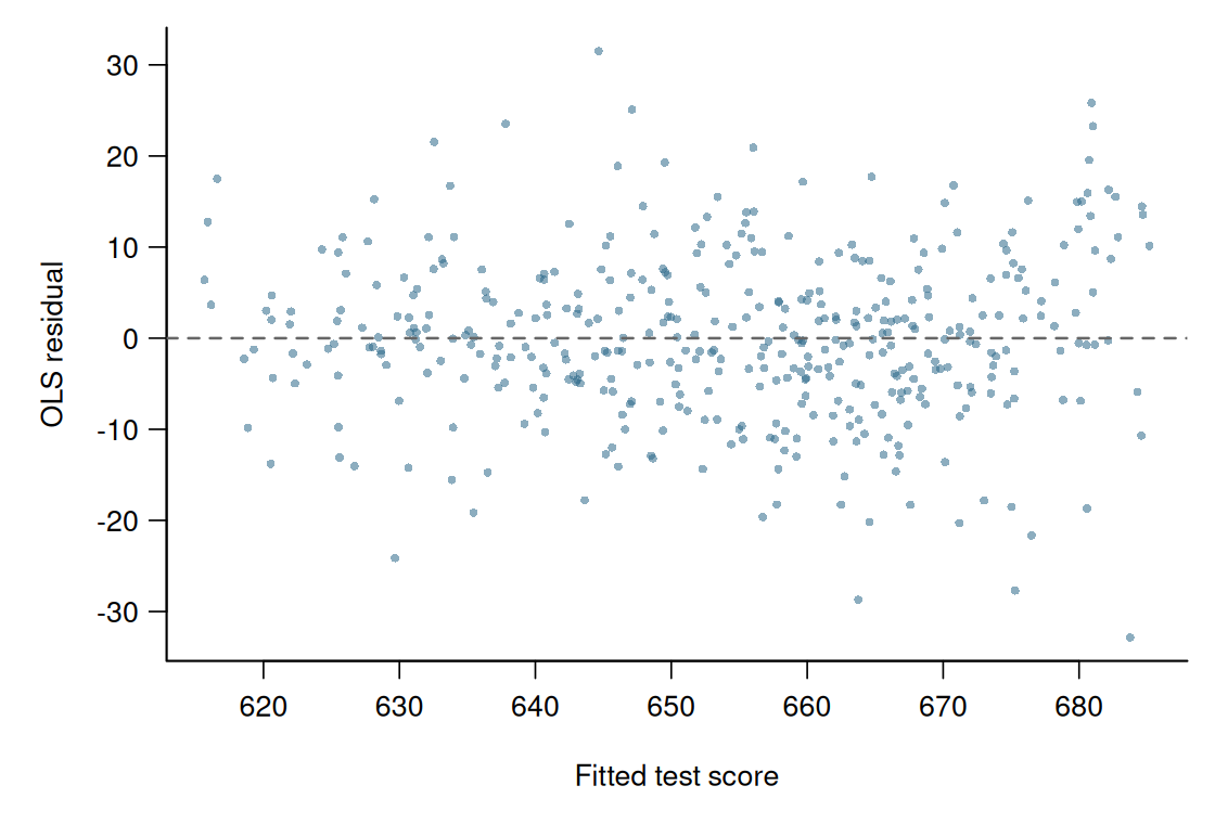
The residuals show no clear systematic pattern around zero, so this plot gives no obvious indication of a misspecified conditional mean.
Heteroskedasticity
Absolute residuals |\widehat u_i| show the size of each deviation without its sign. Plotting them against fitted values gives an overview of changes in the spread.
Patterns related to a particular regressor can remain hidden in this overview. A plot against that regressor can help investigate a specific concern.
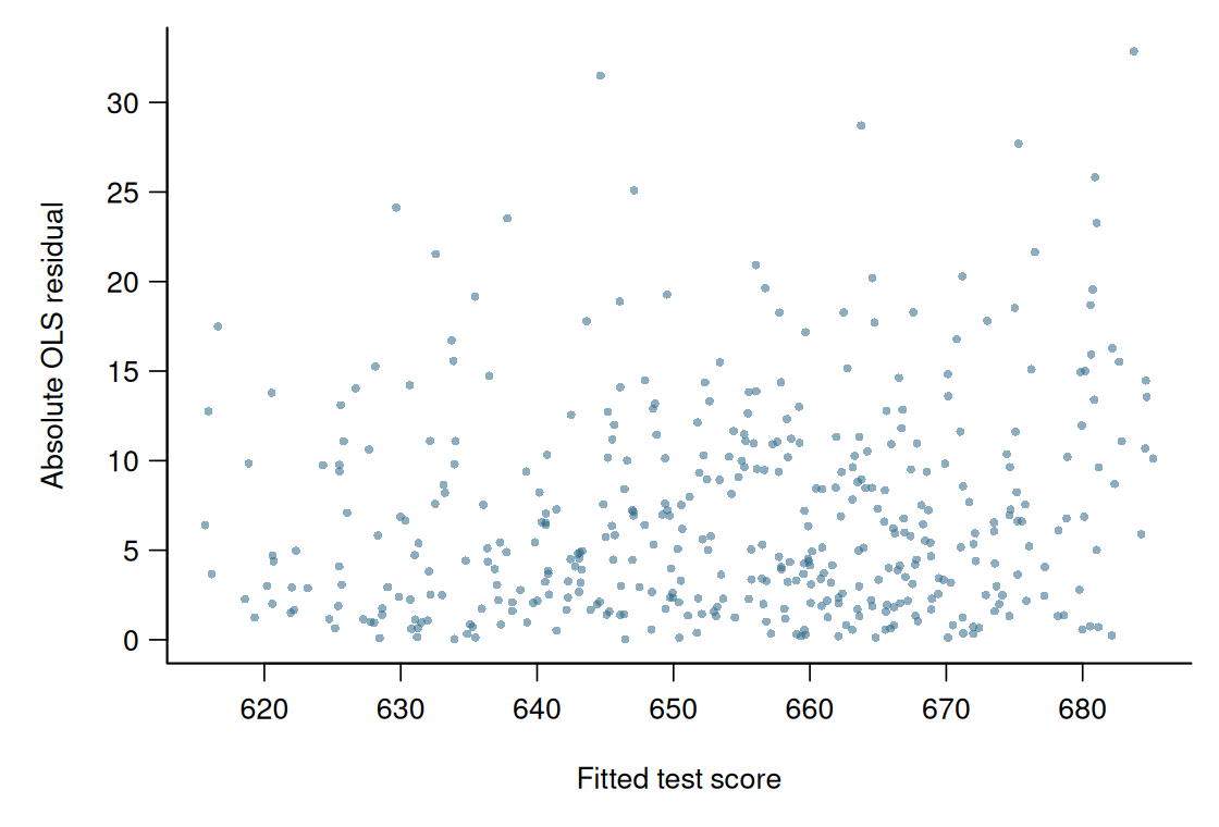
The plot suggests somewhat larger residual magnitudes at higher fitted scores, although the pattern is not pronounced.
Systematic changes in these magnitudes can suggest heteroskedasticity. A misspecified conditional mean can also produce such patterns, so the plot alone does not establish the cause.
Breusch–Pagan Test
The Breusch–Pagan test considers the homoskedasticity hypothesis H_0:\mathrm{Var}(u_i\mid\boldsymbol X_i)=\sigma^2.
Because E[u_i\mid\boldsymbol X_i]=0, the conditional variance equals the conditional second moment. Under homoskedasticity, E[u_i^2\mid\boldsymbol X_i] =\mathrm{Var}(u_i\mid\boldsymbol X_i) =\sigma^2. The population regression of u_i^2 on the regressors therefore has zero slopes.
The test replaces u_i with its OLS residual and runs the auxiliary regression \widehat u_i^2 =\gamma_1+\gamma_2X_{i2}+\cdots+\gamma_kX_{ik}+v_i.
Here, \boldsymbol\gamma contains the auxiliary coefficients. Under homoskedasticity and a correctly specified CEF, the regressors should not systematically predict the squared errors.
Breusch–Pagan Test
Let R_{aux}^2 be the R-squared of the auxiliary regression. The studentized (Koenker) version uses BP=nR_{aux}^2. \tag{7.10}
Under H_0 and the usual large-sample conditions, BP\overset d\to\chi^2_{k-1}.
We reject H_0 at level \alpha if BP>\chi^2_{k-1,1-\alpha}.
Here, k-1 is the number of nonconstant regressors in the auxiliary regression. This version does not require normally distributed errors.
For Model (2), the auxiliary regressors are STR, English learners and subsidized-lunch eligibility:
bptest(class_size_fit, studentize = TRUE)
    studentized Breusch-Pagan test

data:  class_size_fit
BP = 9.9375, df = 3, p-value = 0.0191
The result is BP=9.938, with three degrees of freedom and p-value 0.0191. We reject homoskedasticity at the 5% level.
Under the maintained CEF specification, this provides evidence that the conditional variance changes with the regressors.
For independent observations, HC1 remains the practical default, whether or not a heteroskedasticity test rejects. A failure to reject does not establish homoskedasticity.
Normality
The exact t and F results use the stronger Gaussian assumption from Section 6.9: u_i\mid\boldsymbol X_i\sim\mathcal N(0,\sigma^2).
This specifies both a normal error distribution and a constant conditional variance. We use OLS residuals to look for departures from this model.
Normal Q–Q Plot
A normal Q–Q plot compares the ordered residuals with quantiles of the standard normal distribution.
Writing \widehat u_{(1)}\leq\cdots\leq\widehat u_{(n)} for the ordered residuals, the plotted points are \left(\Phi^{-1}\!\left(\tfrac{i-0.5}{n}\right),\widehat u_{(i)}\right), \qquad i=1,\ldots,n.
If the residual distribution is close to normal, the points should lie approximately on a straight line. Systematic deviations, especially in the tails, suggest a different shape.
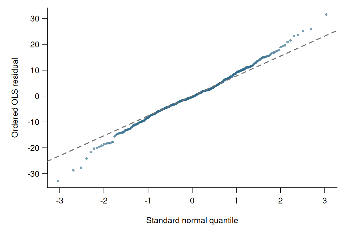
The middle of the plot is close to a straight line, but both tails depart from it. The most extreme residuals are larger in magnitude than the normal reference suggests.
Skewness and Kurtosis
Skewness and kurtosis describe aspects of a distribution’s shape. Skewness measures asymmetry; kurtosis summarizes the importance of large deviations from the mean, often called “tailedness”.
A normal distribution is symmetric, and its tail behaviour is determined by its variance. To compare shapes independently of location and scale, we use moments of the standardized variable (Y-\mu)/\sigma.
Let Y have mean \mu, positive variance \sigma^2 and a finite fourth moment.
Skewness and Kurtosis
The skewness and kurtosis of Y are S=\frac{E[(Y-\mu)^3]}{\sigma^3}, \qquad K=\frac{E[(Y-\mu)^4]}{\sigma^4}.
For a normal distribution, E[(Y-\mu)^3]=0 and E[(Y-\mu)^4]=3\sigma^4. Thus, S=0 and K=3, regardless of its mean and variance.
Skewness summarizes asymmetry. Positive skewness indicates greater weight in the right tail; negative skewness indicates greater weight in the left tail.
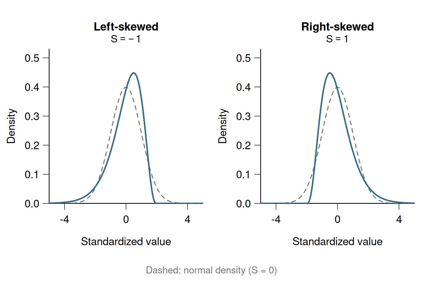
Kurtosis describes the importance of large standardized deviations from the mean. Higher kurtosis indicates a stronger contribution from extreme deviations.
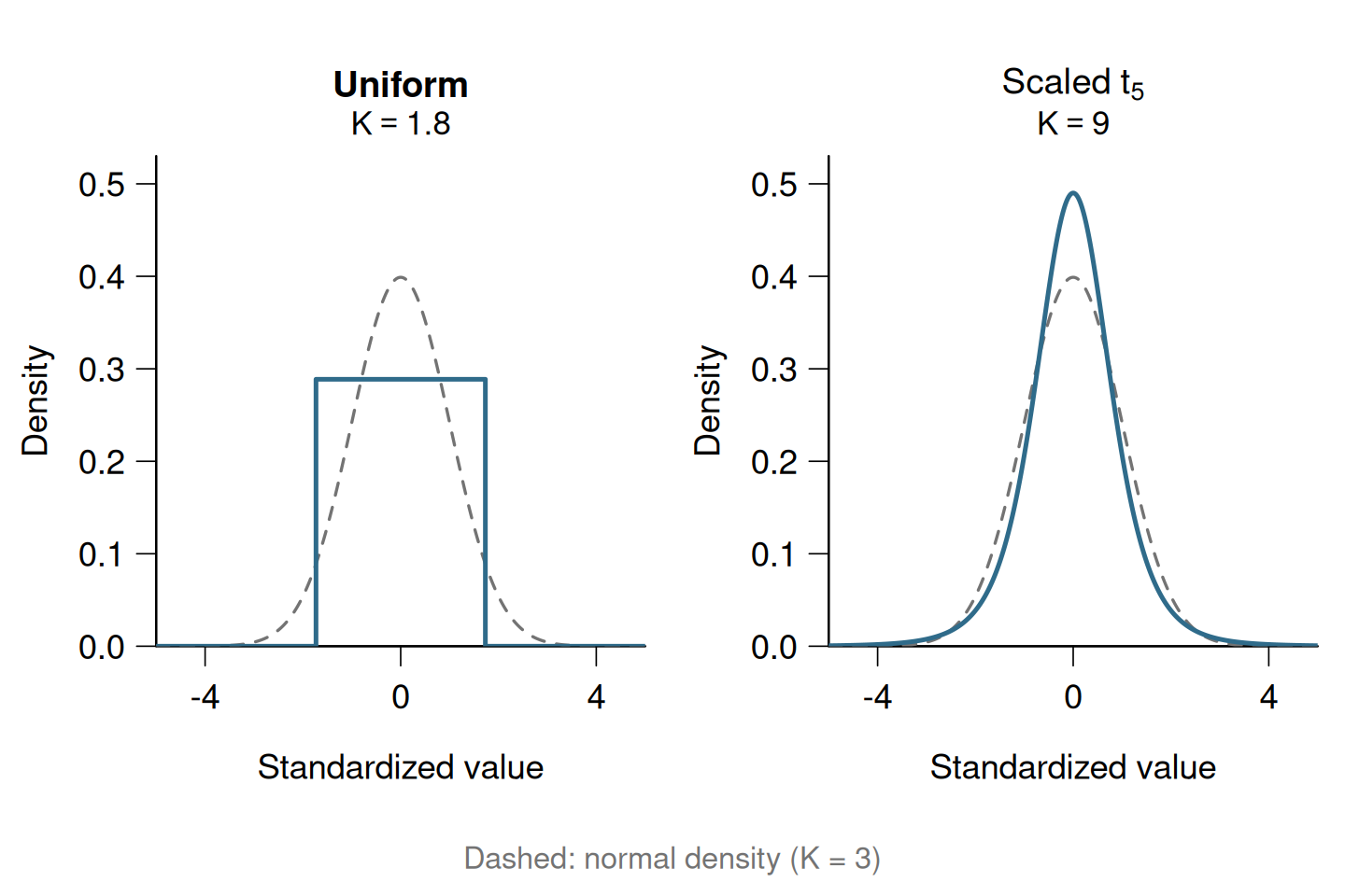
If S=0 and K=3, the first four moments agree with those of a normal distribution with the same mean and variance. This does not establish that the entire distribution is normal.
As in Section 3, we replace population moments with sample moments: \widehat S =\frac{\frac1n\sum_{i=1}^n(Y_i-\overline Y)^3} {\widehat\sigma_Y^3}, \qquad \widehat K =\frac{\frac1n\sum_{i=1}^n(Y_i-\overline Y)^4} {\widehat\sigma_Y^4}, where \widehat\sigma_Y^2=\frac1n\sum_{i=1}^n(Y_i-\overline Y)^2.
For i.i.d. observations with the finite fourth moment and positive variance assumed above, the LLN and the rules for probability limits give \widehat S\overset p\longrightarrow S, \qquad \widehat K\overset p\longrightarrow K.
For regression diagnostics, calculate these quantities from the OLS residuals. With an intercept, their sample mean is zero, so \widehat S_u =\frac{\frac1n\sum_{i=1}^n\widehat u_i^3} {\widehat\sigma_u^3}, \qquad \widehat K_u =\frac{\frac1n\sum_{i=1}^n\widehat u_i^4} {\widehat\sigma_u^4}, where \widehat\sigma_u^2=\frac1n\sum_{i=1}^n\widehat u_i^2.
Jarque–Bera Test
The Jarque–Bera test combines departures of residual skewness from zero and residual kurtosis from three.
Jarque–Bera Test
Using the residual skewness \widehat S_u and kurtosis \widehat K_u, the test statistic is JB=n\left[\frac{\widehat S_u^2}{6} +\frac{(\widehat K_u-3)^2}{24}\right]. \tag{7.11}
Under the homoskedastic Gaussian error model and the usual large-sample conditions, JB\overset d\to\chi_2^2.
We reject at level \alpha if JB>\chi^2_{2,1-\alpha}.
Under the Gaussian null and the same regularity conditions, \widehat S_u and \widehat K_u-3 have approximate variances 6/n and 24/n.
Their standardized versions are asymptotically independent standard normal variables. We can therefore write the statistic as JB= \left(\frac{\widehat S_u}{\sqrt{6/n}}\right)^2 +\left(\frac{\widehat K_u-3}{\sqrt{24/n}}\right)^2.
This is the Wald principle from Section 7.5: standardize departures from the null and combine them, accounting for their covariance. Here, the two standardized components are asymptotically independent, so we add their squares.
The two degrees of freedom correspond to the restrictions S_u=0 and K_u=3.
For the class-size residuals:
   skewness    kurtosis
-0.02359873 3.77781792 jarque.test(uhat)
    Jarque-Bera Normality Test

data:  uhat
JB = 10.626, p-value = 0.004926
alternative hypothesis: greater
The residual skewness is -0.024 and kurtosis is 3.778. Skewness is close to the normal benchmark, while kurtosis is higher.
The result is JB=10.626, with p-value 0.0049. We reject the homoskedastic Gaussian error model at the 1% level.
Changing conditional variances can also make the pooled residual distribution nonnormal. The Q–Q plot and this test do not isolate conditional nonnormality from heteroskedasticity.
Rejecting the Gaussian error model does not, by itself, invalidate the earlier HC1-based large-sample tests. Their validity depends on the assumptions from Section 6, which do not require Gaussian errors.
Leverage and Influence
Section 6.8 distinguishes high leverage from influence: an observation is influential when removing it noticeably changes the fitted regression.
The following plot combines leverage with the absolute OLS residual. Large values on both axes suggest an observation whose influence is worth checking.
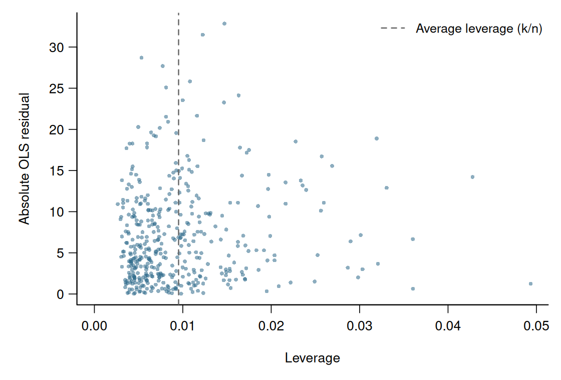
Check unusual observations individually for plausibility and examine whether the main conclusions are sensitive to them. High leverage alone is not a reason to delete an observation.
Section 8 considers which covariance estimator is appropriate when observations are dependent.