set.seed(1)
n = 300
eps = rnorm(n)
WN = ts(eps)
AR1 = filter(eps, 0.8, "recursive")
RW = filter(eps, 1, "recursive")
DT = 1 + 0.2*(1:n) + AR1
par(mfrow = c(2,2))
plot(WN, type = "l")
plot(AR1)
plot(RW)
plot(DT)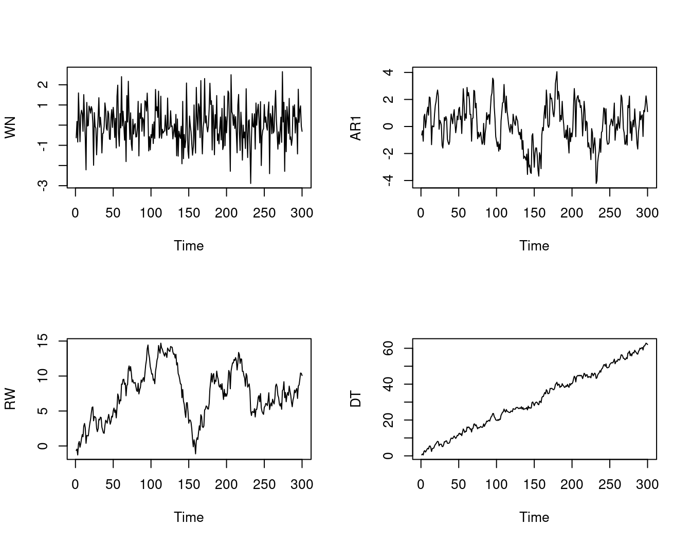
Consider two time series Y_t and Z_t for t=1, \ldots, T. The index t is used instead of i because observations correspond to time points, not individuals. T represents the sample size, i.e., the number of observed time periods.
Some important linear time series regression models:
In these equations, p is the number of lags of the dependent variable Y_t, q is the number of lags of the explanatory variable Z_t, and u_t is a mean zero error (shock) that is conditional mean independent of the regressors.
The coefficients of these models can be estimated by OLS just like in a conventional regression if certain conditions on the time dependence are satisfied.
The AR model can be used for forecasting because the regressors lie in the past relative to the dependent variable. Similarly, the DL and ADL models without the contemporaneous term \delta_0 Z_t can also be used for forecasting. Further exogenous variables can be included as well.
In general, a time series linear regression model is given by Y_t = \boldsymbol X_t'\boldsymbol \beta + u_t, \quad t=1, \ldots, T, where the k-variate vector of regressors \boldsymbol X_t may include exogenous time series and its lags, lags of the dependent variable Y_t, time trends and time dummy variables, and an intercept.
Following the previous identification discussion for the cross-sectional regression model, under exogeneity, E[u_t|\boldsymbol X_t] = 0, for any fixed time t, the population regression coefficient is \boldsymbol \beta = E[\boldsymbol X_t \boldsymbol X_t']^{-1} E[\boldsymbol X_t Y_t]. \tag{9.1}
In order that \boldsymbol \beta in Equation 9.1 makes sense, it must have the same value for all time points t. That is, the second moment matrix E[\boldsymbol X_t \boldsymbol X_t'] and the cross-moment vector E[\boldsymbol X_t Y_t] must be time invariant.
This time invariance property is clearly satisfied if i.i.d. sampling is assumed. However, in time series, i.i.d. is unrealistic because nearby observations are typically dependent (e.g., \mathrm{Cov}(Y_t, Y_{t-1}) \neq 0).
Instead, our time series regression model must allow for time dependencies but also requires this time dependence to be stable over time. A simple way to guarantee that E[\boldsymbol X_t \boldsymbol X_t'] and E[\boldsymbol X_t Y_t] are time invariant is to assume that the joint process (Y_t, \boldsymbol X_t') is (weakly) stationary.
Weak stationarity
A univariate time series Y_t is called (weakly) stationary if its mean and autocovariance are time invariant. That is,
The autocorrelation of order \tau is \rho(\tau) = \frac{\mathrm{Cov}(Y_t, Y_{t-\tau})}{\mathrm{sd}(Y_t) \, \mathrm{sd}(Y_{t-\tau})} = \frac{\gamma(\tau)}{\gamma(0)}, \quad \tau \in \mathbb Z. The autocorrelations of stationary time series typically decay to zero relatively fast as \tau increases, i.e., \rho(\tau) \to 0 as \tau \to \infty. Observations close in time may be highly correlated, but observations farther apart have little dependence.
We define the stationarity concept for multivariate time series analogously:
Multivariate weak stationarity
A multivariate time series \boldsymbol Z_t is (weakly) stationary if
\Gamma(\tau) is the lag-\tau autocovariance matrix.
A time series Y_t is nonstationary if the mean E[Y_t] or the autocovariances Cov(Y_t, Y_{t-\tau}) change with t, i.e., if there exist time points s \neq t with E[Y_t] \neq E[Y_s] \quad \text{or} \quad Cov(Y_t,Y_{t-\tau}) \neq Cov(Y_s,Y_{s-\tau}) for some \tau.
Y_t = \epsilon_t with E[\epsilon_t] = 0, \mathrm{Var}(\epsilon_t) = \sigma^2, and Cov(\epsilon_t, \epsilon_{t-h}) = 0 for all h \neq 0.
Then, \gamma(0) = \sigma^2 and \gamma(\tau) = 0 for \tau \neq 0. White noise is weakly stationary. If \epsilon_t are i.i.d. it is strictly stationary, too.
Y_t = \phi Y_{t-1} + \epsilon_t, where |\phi| < 1 and \epsilon_t is white noise. Y_t is weakly (and under i.i.d. \epsilon_t strictly) stationary with \mu=0,\quad \gamma(0)=\frac{\sigma^2}{1-\phi^2},\quad \rho(\tau)=\phi^{|\tau|}.
Y_t = Y_{t-1} + \epsilon_t, where \epsilon_t is white noise (AR(1) with \phi=1) and Y_0 = 0. It is nonstationary because the variance grows with t: Var(Y_t) = t \sigma^2. But the first difference \Delta Y_t=Y_t-Y_{t-1}=\epsilon_t is stationary.
Nonstationary time series can often be transformed into a stationary time series using an appropriate transformation.
Y_t=\alpha+\beta t+u_t with stationary u_t. Y_t is nonstationary, but removing the deterministic trend (Y_t - \beta t) yields a stationary series.
The sample paths of simulated white noise, AR(1), random walk and deterministic trend time series are shown below. The series shown at the top are stationary while the series at the bottom are nonstationary.
set.seed(1)
n = 300
eps = rnorm(n)
WN = ts(eps)
AR1 = filter(eps, 0.8, "recursive")
RW = filter(eps, 1, "recursive")
DT = 1 + 0.2*(1:n) + AR1
par(mfrow = c(2,2))
plot(WN, type = "l")
plot(AR1)
plot(RW)
plot(DT)
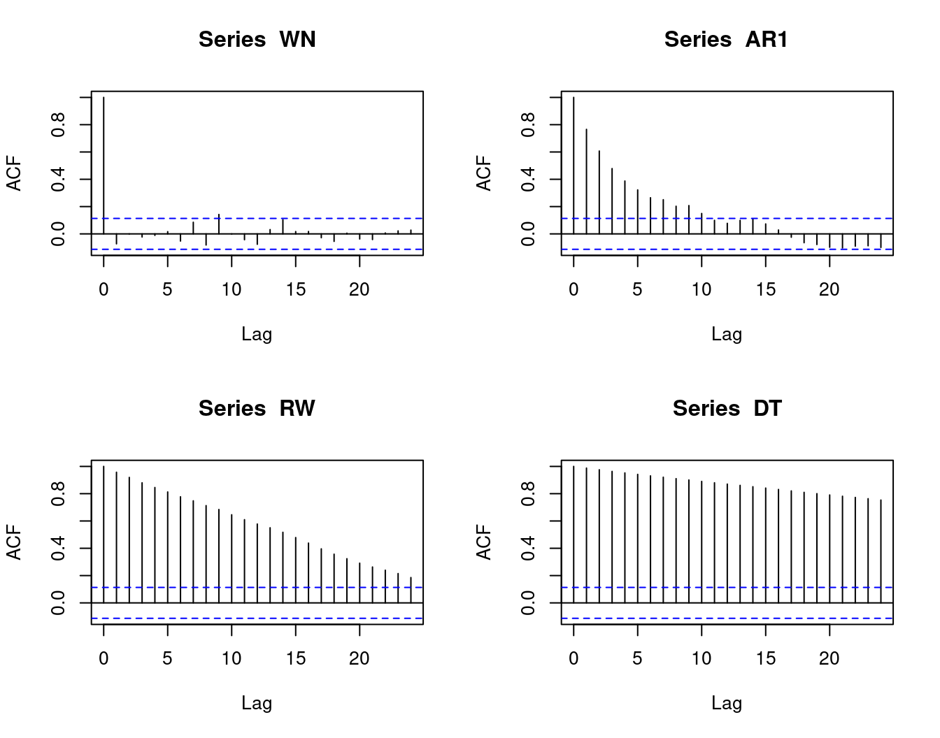
The sample autocovariance function is defined as \widehat \gamma(\tau) = \frac{1}{T} \sum_{t=\tau+1}^T (Y_t - \overline Y)(Y_{t-\tau} - \overline Y), and the sample autocorrelation function (ACF) is \widehat \rho(\tau) = \frac{\widehat \gamma(\tau)}{\widehat \gamma(0)}.
For many stationary time series encountered in practice, the ACF decays to zero quite quickly as \tau increases. The ACFs shown at the top are from stationary time series while the ACFs at the bottom are from nonstationary time series.
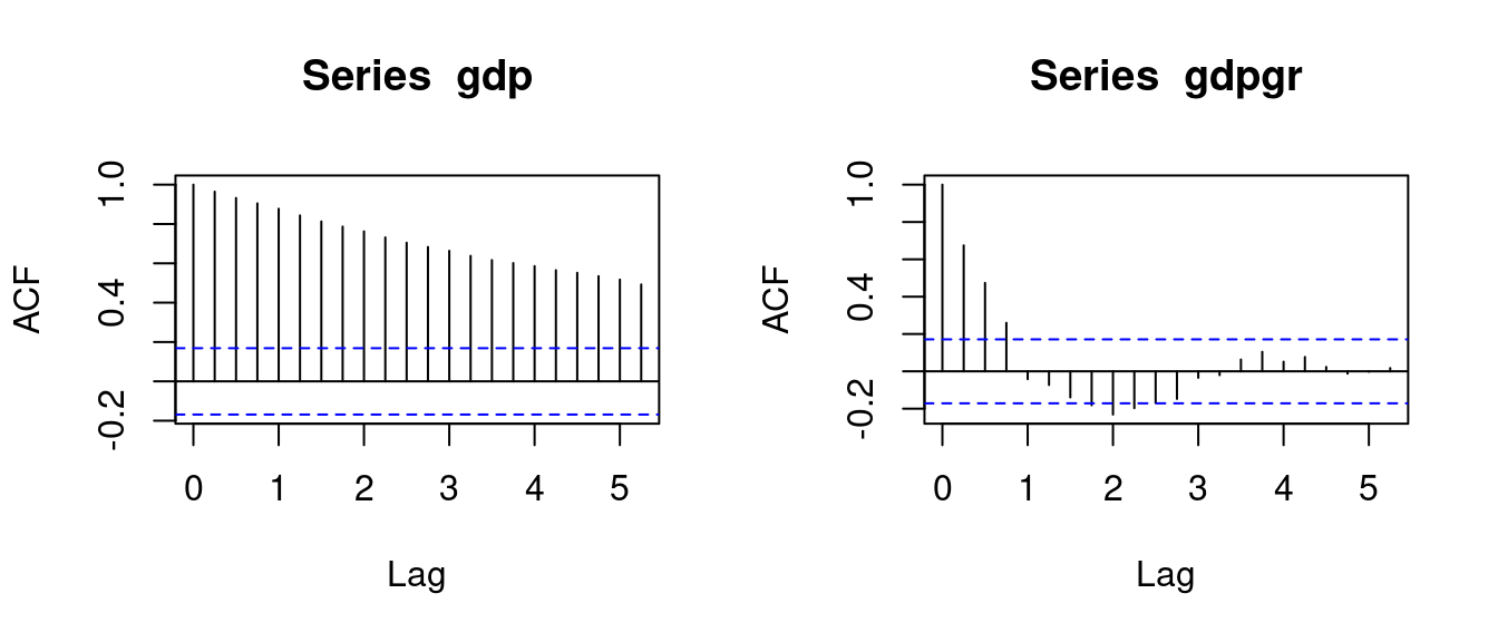
Consider the quarterly nominal GDP of Germany and its annual growth rate:
library(TeachData)
par(mfrow = c(1,2))
plot(gdp, main="Nominal GDP Germany")
gdpgr = diff(log(gdp),4) # annual continuous growth rates of quarterly data
plot(gdpgr, main = "Annual nominal GDP growth")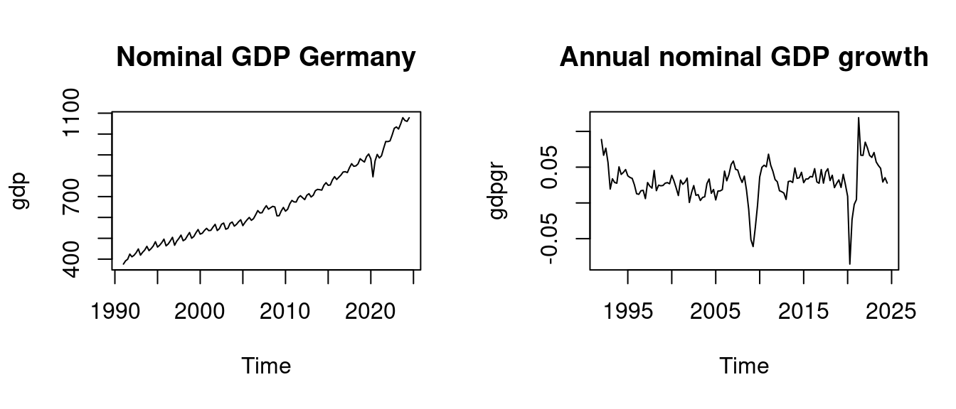
By visual inspection, we observe that the nominal GDP is clearly upward trending and therefore nonstationary. The GDP growth rates show a stationary behavior.
The ACF of nominal GDP decays very slowly and stays close to 1 for many lags, which is typical for nonstationary, trending series. In contrast, the ACF of GDP growth rates drops quickly.
Similarly, the oil price shows nonstationary behavior, while the oil returns (first differences of log-prices) appear stationary:
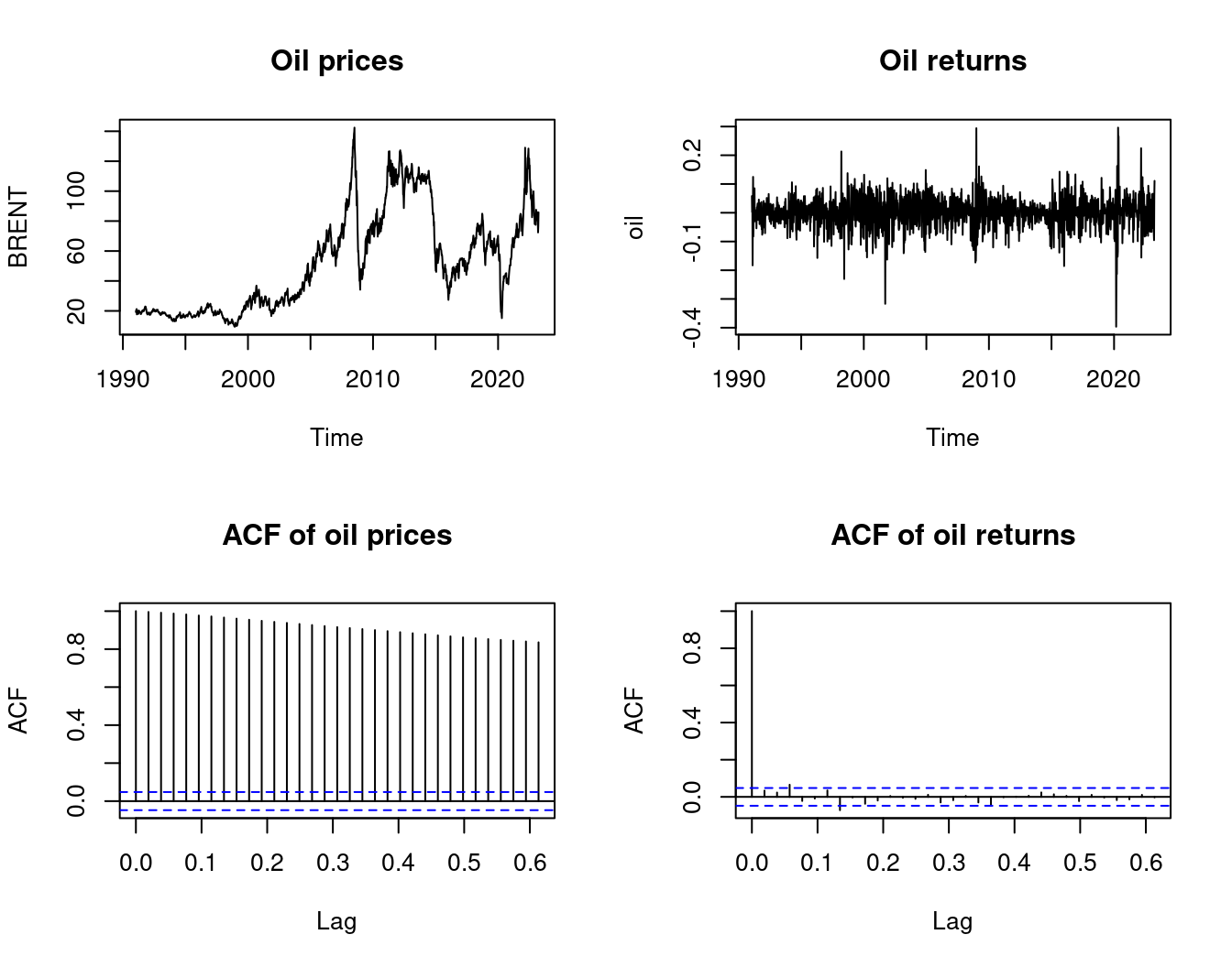
The oil price level shows very persistent correlation, while returns have an ACF that quickly shrinks towards zero.
The returns or continuous growth rates of a time series Y_t are defined as r_t = \Delta \log(Y_t) = \log(Y_t) - \log(Y_{t-1}) = \log\bigg( 1 + \frac{Y_t - Y_{t-1}}{Y_{t-1}} \bigg) \approx \frac{Y_t - Y_{t-1}}{Y_{t-1}}. This approximation holds because \log(1+x) \approx x for x close to 0, which can be shown by a Taylor expansion around 0.
Spurious correlation occurs when two unrelated time series Y_t and X_t have zero population correlation (Cov(Y_t, X_t) = 0) but exhibit a large sample correlation coefficient due to coincidental patterns or trends within the sample data.
Spurious correlations often arise when both series are nonstationary and trending, so that both move in the same or opposite directions over long periods even if there is no dependence.
Here are some examples of nonsense correlations: tylervigen.com/spurious-correlations.
Nonsense correlations may occur if the underlying time series process is nonstationary, particularly in the case of two random walks.
Let’s simulate two independent AR(1) processes: Y_t = \alpha Y_{t-1} + u_t, \quad X_t = \alpha X_{t-1} + v_t, for t=1, \ldots, 300, where u_t and v_t are i.i.d. standard normal. If \alpha = 0.5, the processes are stationary. If \alpha = 1, the processes are nonstationary (random walk).
In any case, the population covariance is zero: Cov(Y_t, X_t) = 0. Therefore, we expect that the sample correlation is zero as well:
set.seed(121)
u = rnorm(300)
v = rnorm(300)
## Two independent AR(1) processes
Y1 = filter(u, 0.5, "recursive")
X1 = filter(v, 0.5, "recursive")
par(mfrow = c(1,2))
plot(Y1, main = "alpha = 0.5")
lines(X1, col="blue")
## Two independent random walks
Y2 = filter(u, 1, "recursive")
X2 = filter(v, 1, "recursive")
plot(Y2, main = "alpha = 1")
lines(X2, col="blue")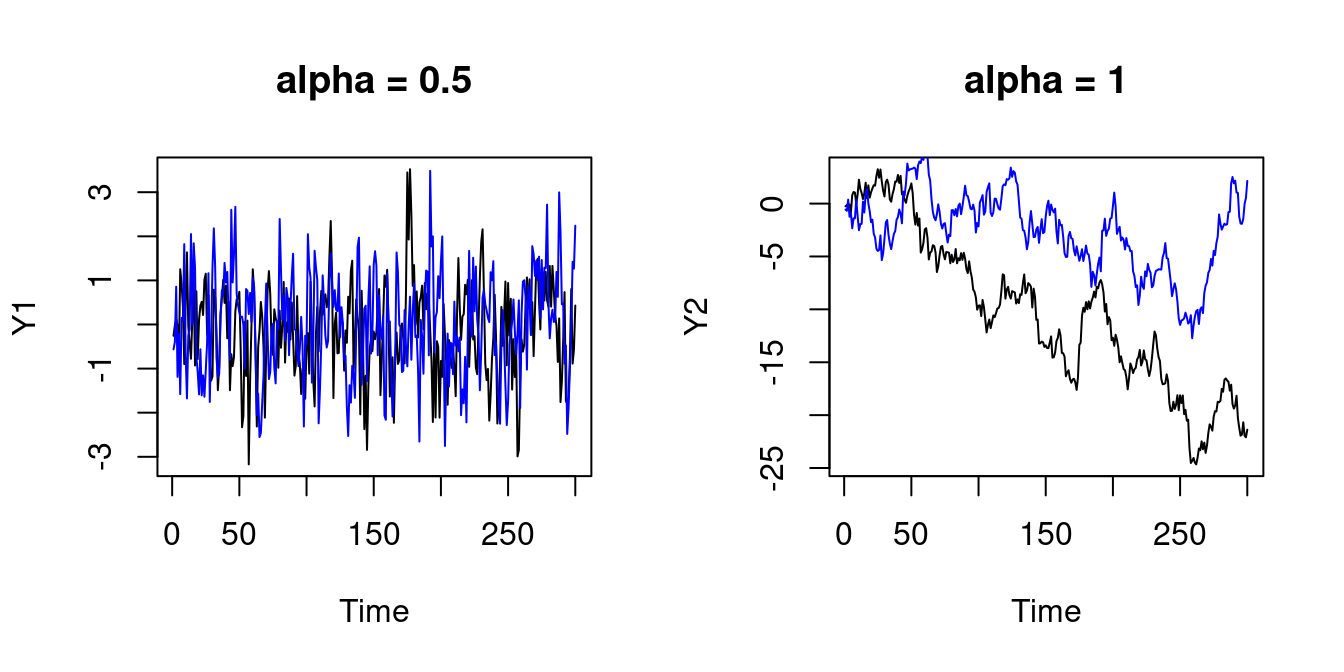
## Sample correlations
c(
  cor(Y1,X1), # alpha = 0.5 (stationary)
  cor(Y2,X2) # alpha = 1 (nonstationary)
)
[1] 0.01077922 0.53448528The sample correlation of the two independent stationary time series is 0.0108 and the sample correlation of the two independent nonstationary time series is 0.5345.
This misleadingly suggests a high correlation between the two series although they are independent and thus have zero population correlation.
The differenced random walk \Delta Y_t = Y_t - Y_{t-1} is stationary, and the sample correlation of the differenced series is close to zero:
It was no coincidence that the two independent random walks exhibited an unusual sample correlation. Let’s repeat the simulation 5 times. In many cases, the sample correlations of two independent nonstationary series are much higher than expected:
## Simulate two independent random walks and their sample correlation
RWcor = function(n){
  u = rnorm(n)
  v = rnorm(n)
  Y = filter(u, 1, "recursive")
  X = filter(v, 1, "recursive")
  return(cor(Y,X))
}
c(RWcor(n=300), RWcor(n=300), RWcor(n=300), RWcor(n=300), RWcor(n=300))
[1] -0.54250305 -0.05513752 -0.19244991 0.14773140 -0.65316903Increasing the sample size to T=1000 gives a similar picture:
c(RWcor(n=1000), RWcor(n=1000), RWcor(n=1000), RWcor(n=1000), RWcor(n=1000))[1] -0.3977535 0.5865576 0.5795633 0.2226966 -0.3157968The reason is that sample correlations and also OLS coefficients are inconsistent if two independent random walks are regressed on each other.
The key problem is that already the sample mean of a random walk is inconsistent. The behavior of the sample mean or OLS coefficients is driven by the stochastic path of the random walk.
Two completely unrelated random walks might share common upward and downward drifts by chance, which can produce high sample correlations although the population correlation is zero.
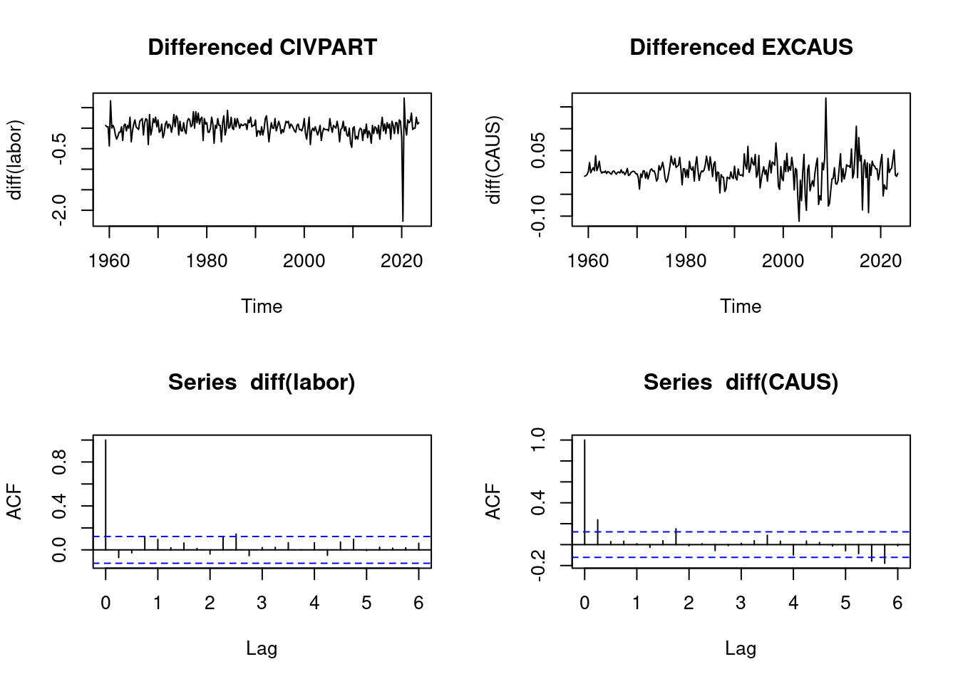
We expect no relationship between the US labor force participation rate and the Canada US exchange rate. However, the sample correlation coefficient is extremely high:
data(fred.qd, package = "TeachData")
labor= na.omit(fred.qd[,"CIVPART"])
CAUS = na.omit(fred.qd[,"EXCAUSx"])
cor(labor, CAUS)
[1] 0.6417728par(mfrow=c(2,2))
plot(labor, main="Labor force participation rate", type = "l")
plot(CAUS, main="Canada US exchange rate", type = "l")
acf(labor)
acf(CAUS)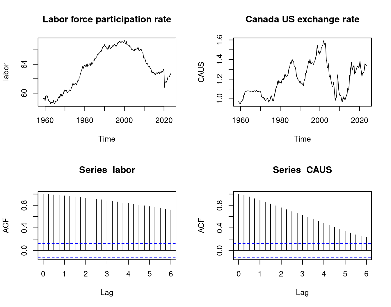
The sample correlation of the differenced series indicates no relationship.
The ACF plot provides a useful tool to decide whether a time series exhibits stationary or nonstationary behavior. We can also run a hypothesis test for the hypothesis that a series is nonstationary against the alternative that it is stationary.
Consider the AR(1) plus constant model: Y_t = c + \phi Y_{t-1} + u_t, \qquad \quad \tag{9.2} where u_t is an i.i.d. zero mean sequence.
Y_t is stationary if |\phi| < 1 and nonstationary if \phi = 1 (the cases \phi > 1 and \phi \leq -1 lead to exponential or oscillating behavior and are ignored here).
Let’s consider the hypotheses \underbrace{H_0: \phi = 1}_{\text{nonstationarity}} \quad vs. \quad \underbrace{H_1: |\phi| < 1}_{\text{stationarity}} To test H_0, we can run a left-sided t-test for the hypothesis \phi = 1. The t-statistic is Z_{\widehat \phi} = \frac{\widehat \phi - 1}{se(\widehat \phi)}, where \widehat \phi is the OLS estimator and se(\widehat \phi) is the homoskedasticity-only standard error.
Unfortunately, under H_0, the time series regression assumptions are not satisfied because Y_t is a random walk. The OLS estimator is not normally distributed, but it is consistent.
It can be shown that the t-statistic does not converge to a standard normal distribution. Instead, it converges to the Dickey-Fuller distribution: Z_{\widehat \phi} \overset{D}{\longrightarrow} DF
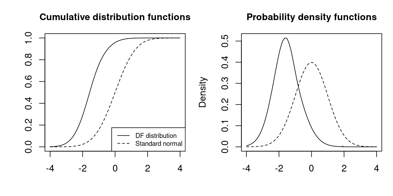
The quantiles of the Dickey-Fuller distribution are much smaller than the normal ones:
| 0.01 | 0.025 | 0.05 | 0.1 | |
|---|---|---|---|---|
| \mathcal N(0,1) | -2.32 | -1.96 | -1.64 | -1.28 |
| DF | -3.43 | -3.12 | -2.86 | -2.57 |
t-statistic lies in the left tail of the Dickey–Fuller distribution (is smaller than the corresponding critical value).
We reject H_0 if the t-statistic Z_{\widehat \phi} is lies in the left tail of the Dickey–Fuller distribution (is smaller than the \alpha quantile from the above table).
Note that here the null hypothesis is nonstationarity (\phi = 1), and the alternative is stationarity (|\phi| < 1).
The assumption that \Delta Y_t = Y_t - Y_{t-1} = u_t in Equation 9.2 is i.i.d. is unreasonable in many cases. It is more realistic that Y_t = c + \phi_1 Y_{t-1} + \ldots + \phi_p Y_{t-p} + u_t for some lag order p. In this model, Y_t is nonstationary if \sum_{j=1}^p \phi_j = 1.
The equation can be rewritten as \Delta Y_t = c + \psi Y_{t-1} + \theta_1 \Delta Y_{t-1} + \ldots + \theta_{p-1} \Delta Y_{t-(p-1)} + u_t, \qquad \quad \tag{9.3} where \psi = \sum_{j=1}^p \phi_j-1 and \theta_i = -\sum_{j=i+1}^p \phi_j.
The lagged differences \Delta Y_{t-j} absorb short-run dynamics so that the remaining error u_t is approximately white noise.
To test for nonstationarity, we formulate the null hypothesis H_0: \sum_{j=1}^p \phi_j = 1, which is equivalent to H_0: \psi = 0.
The t-statistic Z_{\widehat \psi} from Equation 9.3 converges under H_0 to the Dickey-Fuller distribution as well. Therefore, we can reject the null hypothesis of nonstationarity, if Z_{\widehat \psi} is smaller than the corresponding quantile from the DF distribution.
This test is called Augmented Dickey-Fuller test (ADF).
We use the ur.df() function from the urca package with the option type = "drift" to compute the ADF test statistic.
###############################################################
# Augmented Dickey-Fuller Test Unit Root / Cointegration Test #
###############################################################

The value of the test statistic is: 1.9577 6.9976
The ADF statistic Z_{\widehat \psi} is the first value from the output. The critical value for the 5% significance level is -2.86. Hence, the ADF with p = 4 does not reject the null hypothesis that GDP is nonstationary.
ur.df(gdpgr, type = "drift", lags = 4)
###############################################################
# Augmented Dickey-Fuller Test Unit Root / Cointegration Test #
###############################################################

The value of the test statistic is: -4.2971 9.2328
The ADF statistic with p = 4 is below -2.86, and the ADF test rejects the null hypothesis that GDP growth is nonstationary at the 5% significance level.
This matches our earlier graphical evidence: GDP in levels appears nonstationary, while GDP growth behaves like a stationary series.
Let’s come back to our time series regression model Y_t = \boldsymbol X_t'\boldsymbol \beta + u_t, \quad t=1, \ldots, T, where (Y_t, \boldsymbol X_t') is weakly stationary and has finite fourth moments with invertible design matrix E[\boldsymbol X_t \boldsymbol X_t'].
This model has well-specified dynamics if the error u_t contains no systematic predictable component given past information.
A convenient assumption to formalize this is the martingale difference sequence (MDS) property E[u_t | \boldsymbol X_{t}, Y_{t-1}, \boldsymbol X_{t-1}, Y_{t-2}, \boldsymbol X_{t-2}, \ldots] = 0. \tag{9.4}
This implies in particular E[u_t∣\boldsymbol X_t]=0 (exogeneity) and that the errors are uncorrelated over time, E[u_t u_s] = 0 for t \neq s.
Intuitively, the MDS property means that, conditional on the past, u_t is “pure noise”.
Under stationarity, finite fourth moments, and the MDS condition, OLS is consistent and asymptotically normal: \sqrt T (\widehat{\boldsymbol \beta} - \boldsymbol \beta) \overset{d}{\to} \mathcal N(\boldsymbol 0, \boldsymbol Q^{-1} \boldsymbol \Omega \boldsymbol Q^{-1}), \quad \text{as} \ T \to \infty, with \boldsymbol Q and \boldsymbol \Omega as in Section 7.
The asymptotic covariance matrix is the same as in the heteroskedastic case of iid data. Thus, usual HC1/HC3 standard errors, confidence intervals, and t-tests remain valid.
The MDS assumption in Equation 9.4 is plausible if we include enough lags of Y_t as regressor variables.
For example, consider a DL model that explains current gasoline price returns by past oil price returns: \text{gas}_t = \alpha + \delta_1 \text{oil}_{t-1} + \delta_2 \text{oil}_{t-2} + u_t. If gasoline returns are autocorrelated, then u_t must depend on past gasoline prices, which violates Equation 9.4. E.g., u_t may depend on \text{gas}_{t-1} and \text{gas}_{t-2}.
However, in the ADL model that includes the first two lags of the dependent variable to control for that autocorrelation, it is plausible that u_t satisfies Equation 9.4. \text{gas}_t = \alpha + \delta_1 \text{oil}_{t-1} + \delta_2 \text{oil}_{t-2} + \delta_1 \text{gas}_{t-1} + \delta_2 \text{gas}_{t-2} + u_t.
df = ts.union(
  gas = gas,
  oil = oil,
  gas_1 = lag(gas,-1),
  gas_2 = lag(gas,-2),
  oil_1 = lag(oil,-1),
  oil_2 = lag(oil,-2)
)
DLfit = lm(gas ~ oil_1 + oil_2, data = df)
ADLfit = lm(gas ~ oil_1 + oil_2 + gas_1 + gas_2, data = df)
par(mfrow = c(1,2))
acf(DLfit$residuals)
acf(ADLfit$residuals)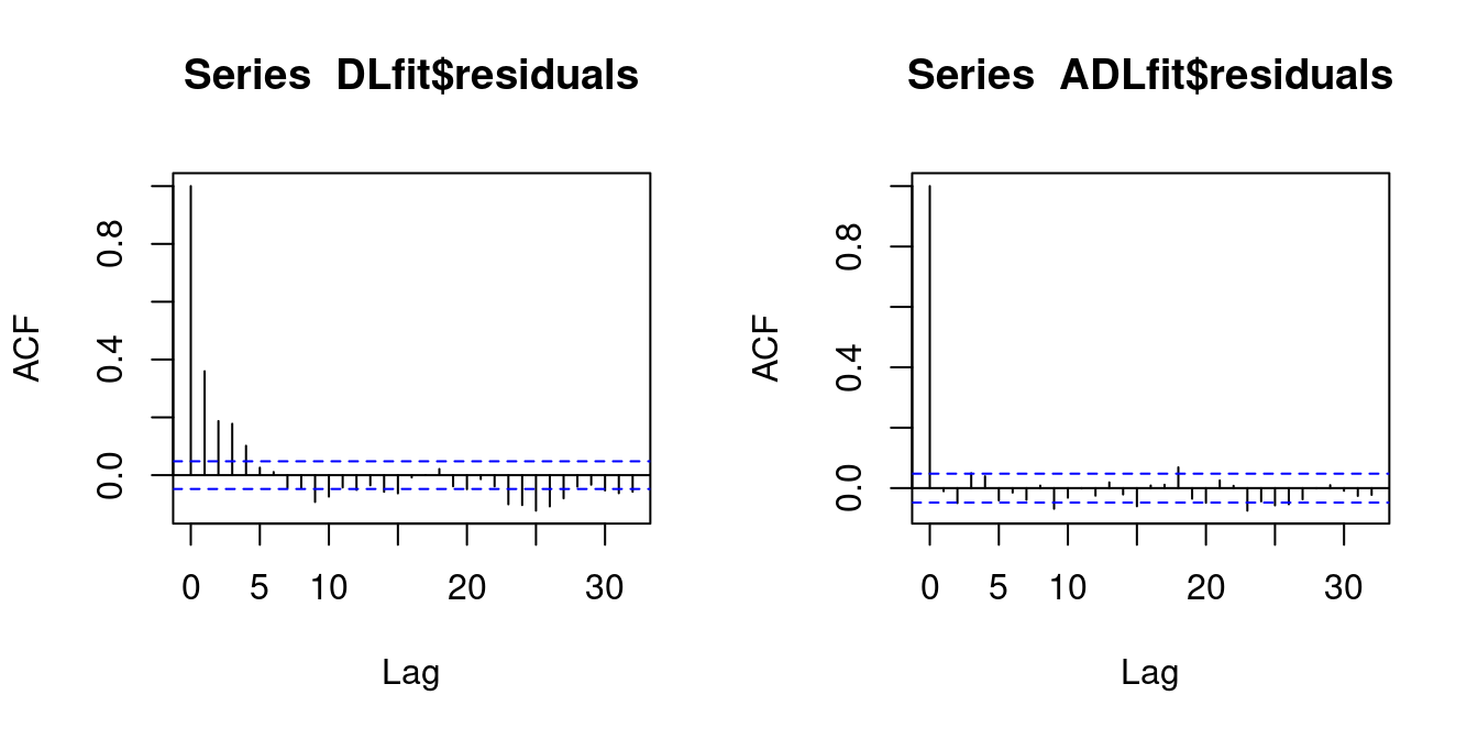
The blue line in the ACF plot indicates the critical values for a test of the hypothesis H_0: \rho(\tau) = 0.
The hypothesis H_0: \rho(1) = 0 is rejected for the residuals of the DL model while the hypothesis is not rejected for the residuals of the ADL model.
Therefore, it is plausible that Equation 9.4 holds for the ADL model while there is strong evidence against it for the DL model.
Thus, using HC1 standard errors seems reasonable for the ADL model. For the DL model, HAC (heteroskedasticity and autocorrelation consistent) standard errors should be used instead.
library(modelsummary)
modelsummary(
  list(DLfit, DLfit, ADLfit),
  vcov = c("HC1", "HAC", "HC1"),
  gof_map = c("nobs", "r.squared", "rmse", "vcov.type")
)| (1) | (2) | (3) | |
|---|---|---|---|
| (Intercept) | 0.000 | 0.000 | 0.000 |
| (0.000) | (0.001) | (0.000) | |
| oil_1 | 0.171 | 0.171 | 0.124 |
| (0.009) | (0.011) | (0.010) | |
| oil_2 | 0.085 | 0.085 | 0.008 |
| (0.010) | (0.011) | (0.011) | |
| gas_1 | 0.375 | ||
| (0.059) | |||
| gas_2 | 0.109 | ||
| (0.043) | |||
| Num.Obs. | 1678 | 1678 | 1678 |
| R2 | 0.258 | 0.258 | 0.398 |
| RMSE | 0.02 | 0.02 | 0.02 |
| Std.Errors | HC1 | HAC | HC1 |
Recall the sampling variance of OLS: \boldsymbol V = \mathrm{Var}(\widehat{\boldsymbol \beta}|\boldsymbol X_1, \ldots, \boldsymbol X_T) = \bigg(\sum_{t=1}^T \boldsymbol X_t \boldsymbol X_t'\bigg)^{-1} \boldsymbol S \, \bigg(\sum_{t=1}^T \boldsymbol X_t \boldsymbol X_t'\bigg)^{-1} with the meat matrix \boldsymbol S = \mathrm{Var}( \sum_{t=1}^T u_t \boldsymbol X_t | \boldsymbol X_1, \ldots, \boldsymbol X_T).
Under i.i.d. sampling or the martingale difference sequence assumption from Equation 9.4, the meat matrix has the form \boldsymbol S = \sum_{t=1}^T E[u_t^2 \boldsymbol X_t \boldsymbol X_t'|\boldsymbol X_1, \ldots, \boldsymbol X_T] = \sum_{t=1}^T \sigma_t^2 \boldsymbol X_t \boldsymbol X_t' with \sigma_t^2 = E[u_t^2|\boldsymbol X_1, \ldots, \boldsymbol X_T]. This result justifies the use of standard heteroskedasticity-robust covariance matrices such as HC1 or HC3.
The Newey-West heteroskedasticity and autocorrelation consistent (HAC) estimator replaces the unknown \Gamma(\tau) by \widehat\Gamma(h) = \frac{1}{T} \sum_{t=h+1}^T \widehat u_t \widehat u_{t-h} \boldsymbol X_t \boldsymbol X_{t-h}'. Furthermore, the summands are downweighted so the estimated meat matrix is defined as follows: \widehat{\boldsymbol S} = T \bigg[ \widehat \Gamma(0) + \sum_{h=1}^{L-1} \Big(1-\frac{h}{L} \Big) \big( \widehat \Gamma(h) + \widehat \Gamma(h)' \big) \bigg], where L is an appropriate truncation parameter that depends on the sample size T.
We introduce the truncation parameter L because, in principle, the true expression involves infinitely many autocovariances, but in finite samples we must cut the lag sum off to control sampling noise at large lags.
L therefore trades off bias (too small L misses relevant autocorrelation) against variance (too large L adds very noisy long-lag terms). In practice one often uses rules of thumb such as L \propto T^{1/4} or L \propto T^{1/3} (with a small constant like 4 in front), or simply chooses a modest L guided by estimated autocorrelations of the residuals.
Then, the Newey-West HAC covariance matrix estimator is \widehat{\boldsymbol V}_{hac} = T \bigg(\sum_{t=1}^T \boldsymbol X_t \boldsymbol X_t'\bigg)^{-1} \bigg( \widehat \Gamma(0) + \sum_{h=1}^{L-1} \Big(1-\frac{h}{L} \Big) \big( \widehat \Gamma(h) + \widehat \Gamma(h)' \big) \bigg) \bigg(\sum_{t=1}^T \boldsymbol X_t \boldsymbol X_t'\bigg)^{-1}.
Even when the dynamics are misspecified (errors autocorrelated), OLS coefficients remain consistent under E[u_t∣X_t]=0, but the usual HC standard errors are no longer valid. HAC/Newey–West corrects the covariance matrix for this autocorrelation.
The HAC standard errors are square roots of the diagonal entries of \widehat{\boldsymbol V}_{hac}. Use these standard errors if regression residuals exhibit autocorrelation but are stationary.