In applied regression analysis, we often want to assess whether a regressor has a statistically significant relationship with the outcome variable (conditional on other regressors).
For instance, in a regression of test scores on the student-teacher ratio, we might be interested in testing whether adding one more student per class has no effect on test scores – that is, whether \beta_j = 0 or not.
A statistical hypothesis is a statement about a parameter of the population distribution.
In hypothesis testing, we divide the parameter space of interest into a null hypothesis and an alternative hypothesis, for instance
\underbrace{H_0:\beta_j = \beta_j^0}_{ \text{null hypothesis} } \quad \text{vs.} \quad \underbrace{H_1:\beta_j \neq \beta_j^0.}_{ \text{alternative hypothesis} }
\tag{8.1}
This idea is not limited to regression coefficients. For any parameter \theta we can test the hypothesis H_0: \theta = \theta_0 against its alternative H_1: \theta \neq \theta_0.
In practice, two-sided alternatives are more common, i.e. H_1: \theta \neq \theta_0, but one-sided alternatives are also possible, i.e. H_1: \theta > \theta_0 (right-sided) or H_1: \theta < \theta_0 (left-sided).
We are interested in testing H_0 against H_1. The idea of hypothesis testing is to construct a statistic T_0 (test statistic) for which the distribution of T_0 under the assumption that H_0 holds (null distribution) is known, and for which the distribution under H_1 differs from the null distribution (i.e., the null distribution is informative about H_1).
If the observed value of T_0 takes a value that is likely to occur under the null distribution, we deduce that there is no evidence against H_0, and consequently we do not reject H_0 (we accept H_0). If the observed value of T_0 takes a value that is unlikely to occur under the null distribution, we deduce that there is evidence against H_0, and consequently, we reject H_0 in favor of H_1.
“Unlikely” means that its occurrence has only a small probability \alpha. The value \alpha is called the significance level and must be selected by the researcher. It is conventional to use the values \alpha \in \{0.1, 0.05, 0.01, 0.001\}, but it is not a hard rule.
A hypothesis test with significance level \alpha is a decision rule defined by a rejection region I_1 and an acceptance region I_0 = I_1^c, where I_1^c is the complement of I_1, so that we \begin{align*}
\text{do not reject} \ H_0 \quad \text{if} \ &T_0 \in I_0, \\
\text{reject} \ H_0 \quad \text{if} \ &T_0 \in I_1.
\end{align*} The rejection region is defined such that a false rejection occurs with probability \alpha, i.e.
P( \underbrace{T_0 \in I_1}_{\text{reject}} \mid H_0 \ \text{is true}) = \alpha,
\tag{8.2} where P(\cdot \mid H_0 \ \text{is true}) denotes the probability function of the null distribution.
A test that satisfies Equation 8.2 is called a size-\alpha-test. The type I error is the probability of falsely rejecting H_0 and equals \alpha for a size-\alpha-test. The type II error is the probability of falsely accepting H_0 and depends on the sample size n and the unknown parameter value \theta under H_1. Typically, the further \theta is from \theta_0, and the larger the sample size n, the smaller the type II error.
The probability of a type I error is also called the size of a test:
P( \text{reject} \ H_0 \mid H_0 \ \text{is true}).
The power of a test is the complementary probability of a type II error:
P( \text{reject} \ H_0 \mid H_1 \ \text{is true}) = 1 - P( \text{accept} \ H_0 \mid H_1 \ \text{is true}).
A hypothesis test is consistent for H_1 if the power tends to 1 as n tends to infinity for any parameter value under the alternative.
Testing Decisions
Accept H_0
Reject H_0
H_0 is true
correct decision
type I error
H_1 is true
type II error
correct decision
In many cases, the probability distribution of T_0 under H_0 is known only asymptotically. Then, the rejection region must be defined such that
\lim_{n \to \infty} P( T_0 \in I_1 \mid H_0 \ \text{is true}) = \alpha.
We call this test an asymptotic size-\alpha-test.
The decision “accept H_0” does not mean that H_0 is true. Since the probability of a type II error is unknown in practice, it is more accurate to say that we “fail to reject H_0” instead of “accept H_0”. The power of a consistent test tends to 1 as n increases, so type II errors typically occur if the sample size is too small. Therefore, to interpret a “fail to reject H_0”, we have to consider whether our sample size is relatively small or rather large.
8.2 t-Test
The most common hypothesis test evaluates whether a regression coefficient equals zero:
H_0: \beta_j = 0 \quad \text{vs.} \quad H_1: \beta_j \ne 0.
This corresponds to testing whether the marginal effect of the regressor X_{ij} on the outcome Y_i is zero, holding other regressors constant.
We use the t-statistic:
T_j = \frac{\widehat{\beta}_j}{\mathrm{se}(\widehat{\beta}_j)},
where se(\widehat{\beta}_j) is a standard error.
You may use the classical standard error if you have strong evidence that the errors are homoskedastic. However, in most economic applications, heteroskedasticity-robust standard errors are more reliable.
Under the null, T_j follows approximately a t_{n-k} distribution. We reject H_0 at the significance level \alpha if:
|T_j| > t_{n-k,1-\alpha/2}.
This decision rule is equivalent to checking whether the confidence interval for \beta_j includes 0:
Reject H_0 if 0 lies outside the 1-\alpha confidence interval
Fail to reject (accept) H_0 if 0 lies inside the 1-\alpha confidence interval
8.3 p-Value
The p-value is a criterion to reach a hypothesis test decision conveniently: \begin{align*}
\text{reject} \ H_0 \quad &\text{if p-value} < \alpha \\
\text{do not reject} \ H_0 \quad &\text{if p-value} \geq \alpha
\end{align*}
Formally, the p-value represents the probability of observing a test statistic as extreme or more extreme than the one we computed, assuming H_0 is true. For the t-test, the p-value is:
p\text{-value} = P( |S| > |T_j| \mid H_0 \ \text{is true})
Here, S is a random variable following the null distribution S\sim t_{n-k}, and T_j is the observed value of the test statistic.
Another way of writing the p-value of a t-test is:
p\text{-value} = 2(1 - F_{t_{n-k}}(|T_j|)),
where F_{t_{n-k}} is the cumulative distribution function (CDF) of the t_{n-k}-distribution.
The reason is that, by the symmetry of the t-distribution, \begin{align*}
p\text{-value} &= P(|S| > |T_j| \mid H_0 \ \text{is true}) \\
&= 1 - P(|S| \leq |T_j| \mid H_0 \ \text{is true}) \\
&= 1 - F_{t_{n-k}}(|T_j|) + F_{t_{n-k}}(-|T_j|) \\
&= 2(1 - F_{t_{n-k}}(|T_j|)).
\end{align*}
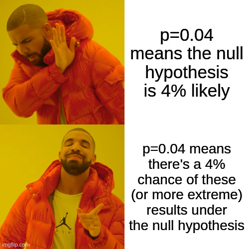
A common misinterpretation of p-values is treating them as the probability that the null hypothesis is being true. This is incorrect. The p-value is not a statement about the probability of the null hypothesis itself.
The correct interpretation is that the p-value represents the probability of observing a test statistic at least as extreme as the one calculated from our sample, assuming that the null hypothesis is true.
In other words, a p-value of 0.04 means:
❌ NOT “There’s a 4% chance that the null hypothesis is true”
✓ INSTEAD “If the null hypothesis were true, there would be a 4% chance of observing a test statistic this extreme or more extreme”
Small p-values indicate that the observed data would be unlikely under the null hypothesis, which leads us to reject the null in favor of the alternative. However, they do not tell us the probability that our alternative hypothesis is correct, nor do they directly measure the magnitude or significance of the marginal effect.
Relation to Confidence Intervals:
Zero lies outside the (1-\alpha) confidence interval for \beta_j if and only if the p-value for testing H_0: \beta_j = 0 is less than \alpha.
8.4 Significance Stars
Regression tables often use asterisks to indicate levels of statistical significance. Stars summarize statistical significance by comparing the t-statistic to critical values (or equivalently, the p-value or whether 0 is covered by the confidence interval)
0 outside \small I_{0.9}, but inside \small I_{0.95}
Significance Stars Convention
Note that most economists use the following significance levels: *** for 1%, ** for 5%, and * for 10%. However, the default convention within R is: *** for 0.1%, ** for 1%, and * for 5%. Therefore, we set the stars manually in the modelsummary() function to match the common economic convention.
Regression Tables
Let’s revisit the regression of wage on education and female.
Let’s also revisit the CASchools dataset and examine four regression models on test scores.
library(AER)data(CASchools, package ="AER")CASchools$STR=CASchools$students/CASchools$teachersCASchools$score=(CASchools$read+CASchools$math)/2fitA=lm(score~STR, data =CASchools)fitB=lm(score~STR+english, data =CASchools)fitC=lm(score~STR+english+lunch, data =CASchools)fitD=lm(score~STR+english+lunch+expenditure, data =CASchools)
Models A–C: The coefficient is negative and statistically significant. However, when using robust standard errors, the coefficient in model B becomes only weakly significant.
Model D: The coefficient remains negative but becomes insignificant when controlling for expenditure.
As discussed earlier, expenditure is a bad control in this context and should not be used to estimate a ceteris paribus effect of class size on test scores.
A concise summary of the regression results with robust standard errors can also be obtained using the coeftest() function from the lmtest package, which is part of the AER package.
t test of coefficients:

               Estimate  Std. Error  t value  Pr(>|t|)
(Intercept)  6.6599e+02  1.0377e+01  64.1803 < 2.2e-16 ***
STR         -2.3539e-01  3.2481e-01  -0.7247 0.4690542
english     -1.2834e-01  3.2440e-02  -3.9563 8.951e-05 ***
lunch       -5.4639e-01  2.3169e-02 -23.5834 < 2.2e-16 ***
expenditure  3.6220e-03  9.4474e-04   3.8339 0.0001457 ***
---
Signif. codes:  0 '***' 0.001 '**' 0.01 '*' 0.05 '.' 0.1 ' ' 1
8.5 Testing for Heteroskedasticity: Breusch-Pagan Test
Classical standard errors should only be used if you have statistical evidence that the errors are homoskedastic. A statistical test for this is the Breusch-Pagan Test.
Under homoskedasticity, the variance of the error term is constant and does not depend on the values of the regressors:
\mathrm{Var}(u_i | \boldsymbol X_i) = \sigma^2 \quad \text{(constant)}.
To test this assumption, we perform an auxiliary regression of the squared residuals on the original regressors:
\widehat u_i^2 = \boldsymbol X_i' \boldsymbol \gamma + v_i, \quad i = 1, \ldots, n,
where:
\widehat u_i are the OLS residuals from the original model,
\boldsymbol \gamma are auxiliary coefficients,
v_i is the error term in the auxiliary regression.
If homoskedasticity holds, the regressors should not explain any variation in \widehat u_i^2, which means the auxiliary regression should have low explanatory power.
Let R^2_{\text{aux}} be the R-squared from this auxiliary regression. Then, the Breusch–Pagan (BP) test statistic is:
BP = n \cdot R^2_{\text{aux}}
Under the null hypothesis of homoskedasticity,
H_0: \mathrm{Var}(u_i | \boldsymbol X_i) = \sigma^2,
the test statistic follows an asymptotic chi-squared distribution with k-1 degrees of freedom:
BP \overset{d}{\rightarrow} \chi^2_{k-1}
We reject H_0 at significance level \alpha if:
BP > \chi^2_{1-\alpha,\,k-1}.
This basic variant of the BP test is Koenker’s version of the test. Other variants include further nonlinear transformations of the regressors.
In R, the test is implemented via the bptest() function from the lmtest package, which is part of the AER package.
    studentized Breusch-Pagan test

data:  fitC
BP = 9.9375, df = 3, p-value = 0.0191
fitD|>bptest()# score on STR, english, lunch, expenditure
    studentized Breusch-Pagan test

data:  fitD
BP = 5.9649, df = 4, p-value = 0.2018
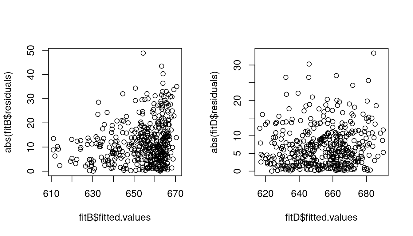
In the regression of score on STR and english there is strong statistical evidence that errors are heteroskedastic, whereas when adding lunch and expenditure there is no evidence of heteroskedasticity. See the difference in the absolute residuals against fitted values plot:
The heteroskedasticity pattern in model (2) likely occurred because of a nonlinear dependence of the omitted variables lunch and expenditure with the included regressors STR and english. The inclusion of these variables in model (4) eliminated the heteroskedasticity (apparent heteroskedasticity). Therefore, heteroskedasticity is sometimes a sign of model misspecification.
8.6 Testing for Normality: Jarque–Bera Test
A general property of a normally distributed variable is that it has zero skewness and kurtosis of three. In the Gaussian regression model, this implies:
u_i|\boldsymbol X_i \sim \mathcal{N}(0, \sigma^2) \quad \Rightarrow \quad E[u_i^3] = 0, \quad E[u_i^4] = 3 \sigma^4.
The sample skewness and sample kurtosis of the OLS residuals are:
\widehat{\text{skew}}(\widehat{\boldsymbol u}) = \frac{1}{n \widehat \sigma_{\widehat u}^3} \sum_{i=1}^n \widehat u_i^3, \quad
\widehat{\text{kurt}}(\widehat{\boldsymbol u}) = \frac{1}{n \widehat \sigma_{\widehat u}^4} \sum_{i=1}^n \widehat u_i^4
A joint test for normality — assessing both skewness and kurtosis — is the Jarque–Bera (JB) test, with statistic:
JB = n \left( \frac{1}{6} \widehat{\text{skew}}(\widehat{\boldsymbol u})^2 + \frac{1}{24} (\widehat{\text{kurt}}(\widehat{\boldsymbol u}) - 3)^2 \right)
Under the null hypothesis of normal errors, this test statistic is asymptotically chi-squared distributed:
JB \overset{d}{\to} \chi^2_2
We reject H_0 at level \alpha if:
JB > \chi^2_{1-\alpha,\,2}.
In R, we can apply the test using the moments package:
    Jarque-Bera Normality Test

data:  fitD$residuals
JB = 8.9614, p-value = 0.01133
alternative hypothesis: greater
Although the Breusch–Pagan test does not reject homoskedasticity for fitD (so classical standard errors are valid asymptotically), the JB rejects the null hypothesis of normal errors at the 5% level and provides statistical evidence that the errors are not normally distributed.
This means that exact inference based on t-distributions is not valid in finite samples, and confidence intervals or t-test results give only large sample approximations.
In econometrics, asymptotic large sample approximations have become the convention because exact finite sample inference is rarely feasible.
8.7 Joint Hypothesis Testing
So far, we’ve tested whether a single coefficient is zero. But often we want to test multiple restrictions simultaneously, such as whether a group of variables has a joint effect.
The joint exclusion hypothesis formulates the null hypothesis that a set of coefficients or linear combinations of coefficients are equal to zero:
H_0: \boldsymbol{R}\boldsymbol{\beta} = \boldsymbol{0}
where:
\boldsymbol{R} is a q \times k restriction matrix,
\boldsymbol{0} is the q \times 1 vector of zeros,
q is the number of restrictions.
Consider for example the score on STR regression with interaction effects:
\text{score}_i = \beta_1 + \beta_2 \text{STR}_i + \beta_3 \text{HiEL}_i + \beta_4 \text{STR}_i \cdot \text{HiEL}_i + u_i.
## Create dummy variable for high proportion of English learnersCASchools$HiEL=(CASchools$english>=10)|>as.numeric()fitE=lm(score~STR+HiEL+STR:HiEL, data =CASchools)fitE|>coeftest(vcov =vcovHC, type ="HC1")
t test of coefficients:

             Estimate Std. Error t value Pr(>|t|)
(Intercept) 682.24584   11.86781 57.4871   <2e-16 ***
STR          -0.96846    0.58910 -1.6440   0.1009
HiEL          5.63914   19.51456  0.2890   0.7727
STR:HiEL     -1.27661    0.96692 -1.3203   0.1875
---
Signif. codes:  0 '***' 0.001 '**' 0.01 '*' 0.05 '.' 0.1 ' ' 1
The model output reveals that none of the individual t-tests reject the null hypothesis that the individual coefficients are zero.
However, these results are misleading because the true marginal effects are a mixture of these coefficients:
\frac{\partial E[\text{score}_i \mid \boldsymbol X_i]}{\partial \text{STR}_i} = \beta_2 + \beta_4 \cdot \text{HiEL}_i.
Therefore, to test if STR has an effect on score, we need to test the joint hypothesis:
H_0: \beta_2 = 0 \quad \text{and} \quad \beta_4 = 0.
In terms of the multiple restriction notation H_0: \boldsymbol{R} \boldsymbol{\beta} = \boldsymbol{0}, we have
\boldsymbol{R} = \begin{pmatrix}
0 & 1 & 0 & 0 \\
0 & 0 & 0 & 1
\end{pmatrix}.
Similarly, the marginal effect of HiEL is:
\frac{\partial E[\text{score}_i \mid \boldsymbol X_i]}{\partial \text{HiEL}_i} = \beta_3 + \beta_4 \cdot \text{STR}_i.
We test the joint hypothesis that \beta_3 = 0 and \beta_4 = 0:
\boldsymbol{R} = \begin{pmatrix}
0 & 0 & 1 & 0 \\
0 & 0 & 0 & 1
\end{pmatrix}.
Wald Test
The Wald test is based on the Wald distance:
\boldsymbol{d} = \boldsymbol{R} \widehat{\boldsymbol{\beta}},
which measures how far the estimated coefficients deviate from the hypothesized restrictions.
The covariance matrix of the Wald distance is: Var(\boldsymbol{d} | \boldsymbol X) = \boldsymbol{R} Var(\widehat{\boldsymbol \beta} | \boldsymbol X) \boldsymbol R', which can be estimated as:
\widehat{Var}(\boldsymbol{d} \mid \boldsymbol X) = \boldsymbol{R} \widehat{\boldsymbol{V}} \boldsymbol{R}'.
The Wald statistic is the squared, variance-standardized distance:
W = \boldsymbol{d}' (\boldsymbol{R} \widehat{\boldsymbol{V}} \boldsymbol{R}')^{-1} \boldsymbol{d},
where \widehat{\boldsymbol{V}} is a consistent estimator of the covariance matrix of \widehat{\boldsymbol{\beta}} (e.g., HC1 robust: \widehat{\boldsymbol{V}} = \widehat{\boldsymbol{V}}_{hc1}).
Under the null hypothesis and the standard assumptions for the heteroskedastic linear model, the Wald statistic has an asymptotic chi-squared distribution:
W \overset{d}{\to} \chi^2_q,
where q is the number of restrictions.
The null is rejected if W > \chi^2_{1-\alpha, q}.
F-test
The Wald test is an asymptotic size-\alpha-test. Even if normality and homoskedasticity hold true, the Wald test is still only asymptotically valid, i.e.:
\lim_{n \to \infty} P( \text{Wald test rejects} \ H_0 | H_0 \ \text{true} ) = \alpha.
The F-test is the small sample correction of the Wald test. It is based on the same distance as the Wald test, but it is scaled by the number of restrictions q:
F = \frac{W}{q} = \frac{1}{q} (\boldsymbol R\widehat{\boldsymbol \beta})'(\boldsymbol R \widehat{\boldsymbol V} \boldsymbol R')^{-1} (\boldsymbol R\widehat{\boldsymbol \beta}).
Under the restrictive assumption that the Gaussian regression model holds, and if \widehat{\boldsymbol V} = \widehat{\boldsymbol V}_{hom} is used, it can be shown that
F \sim F_{q,n-k}
for any finite sample size n. Here, F_{q,n-k} is the F-distribution with q degrees of freedom in the numerator and n-k degrees of freedom in the denominator.
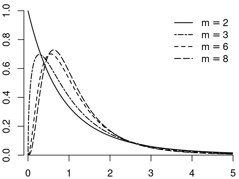
F-distribution
If Q_1 \sim \chi^2_m and Q_2 \sim \chi^2_r, and if Q_1 and Q_2 are independent, then
Y = \frac{Q_1/m}{Q_2/r}
is F-distributed with parameters m and r, written Y \sim F_{m,r}.
The parameter m is called the numerator degree of freedom; r is the denominator degree of freedom.
If r \to \infty then the distribution of mY approaches \chi^2_m
Figure 8.1: F-distribution
F-test decision rule
The test decision for the F-test: \begin{align*}
\text{do not reject} \ H_0 \quad \text{if} \ &F \leq F_{(1-\alpha,q,n-k)}, \\
\text{reject} \ H_0 \quad \text{if} \ &F > F_{(1-\alpha,q,n-k)},
\end{align*} where F_{(p,m_1,m_2)} is the p-quantile of the F distribution with m_1 degrees of freedom in the numerator and m_2 degrees of freedom in the denominator.
F- and Chi-squared distribution
Similar to how the t-distribution t_{n-k} approaches the standard normal as sample size increases, we have q \cdot F_{q,n-k} \to \chi^2_{q} as n \to \infty. Therefore, the F-test and Wald test become asymptotically equivalent and lead to identical statistical conclusions in large samples. For single constraint (q=1) hypotheses of the form H_0: \beta_j = 0, the F-test is equivalent to a two-sided t-test.
The F-test can be viewed as a finite-sample correction of the Wald test. It tends to be more conservative than the Wald test in small samples, meaning that rejection by the F-test generally implies rejection by the Wald test, but not necessarily vice versa. Due to this more conservative nature, which helps control false rejections (Type I errors) in small samples, the F-test is often preferred in practice.
F-tests in R
You can use the function linearHypothesis() from the car package (part of the AER package) to perform a F-test:
linearHypothesis(fitE, c("STR = 0", "STR:HiEL = 0"), vcov =vcovHC(fitE, type ="HC1"), test ="F")
The hypotheses that STR and HiEL have no effect on score is rejected at the 1% level.
Another research question is whether the effect of STR on score is zero only for the subgroup of schools with a high proportion of English learners (HiEL = 1). In this case, the marginal effect is:
\frac{\partial E[\text{score}_i \mid \boldsymbol X_i, \text{HiEL}_i = 1]}{\partial \text{STR}_i} = \beta_2 + \beta_4 \cdot 1,
and the null hypothesis is:
H_0: \beta_2 + \beta_4 = 0.
Similarly, this hypothesis can be rejected at the 1% level.
It is also possible to directly supply the corresponding restriction matrix. For this hypothesis, the restriction matrix is:
\boldsymbol{R} = \begin{pmatrix}
0 & 1 & 0 & 1
\end{pmatrix},
where the number of restrictions is q=1.
R=matrix(c(0,1,0,1), ncol =4)# restriction matrixlinearHypothesis(fitE, hypothesis.matrix =R, vcov =vcovHC(fitE, type ="HC1"), test ="F")