cps = read.csv("cps.csv")
exper = cps$experience
wage = cps$wage
edu = cps$education
fem = cps$female2 Sample distribution
In statistics, a univariate dataset Y_1, \ldots, Y_n or a multivariate dataset \boldsymbol X_1, \ldots, \boldsymbol X_n is often called a sample because it typically represents observations selected from a larger population. The sample distribution indicates how the sample values are distributed across possible outcomes. Summary statistics, such as the sample mean and sample variance, provide a concise representation of key characteristics of the sample distribution.
2.1 Empirical distribution function
The sample distribution of a univariate sample Y_1, \ldots, Y_n is represented by the empirical cumulative distribution function (ECDF), which shows the proportion of observations in the sample that are less than or equal to a certain value a. There are two equivalent ways to define the ECDF: using the indicator function and using order statistics.
Indicator function
The indicator function I(\cdot) is defined as: I(Y_i \leq a) = \begin{cases} 1 & \text{if} \ Y_i \leq a, \\ 0 & \text{if} \ Y_i > a. \end{cases} The ECDF is defined as: \widehat{F}(a) = \frac{1}{n} \sum_{i=1}^n I(Y_i \leq a). This formula calculates the proportion of sample observations that are less than or equal to the value a.
Order statistics
Equivalently, the ECDF can be defined using order statistics. Order statistics are the sample data arranged in ascending order: Y_{(1)} \leq Y_{(2)} \leq \ldots \leq Y_{(n)}. In R, you can compute the order statistics of a univariate data vector Y using the command sort(Y). The ECDF is then defined as:
\widehat{F}(a) =
\begin{cases}
0 & \text{if } a < Y_{(1)}, \\
\frac{k}{n} & \text{if } Y_{(k)} \leq a < Y_{(k+1)}, \quad k = 1, 2, \ldots, n - 1, \\
1 & \text{if } a \geq Y_{(n)}.
\end{cases}
The ECDF is a step function that increases by 1/n at each data point Y_{(k)}. The function remains constant between data points and jumps at each observed value in the sample.
Some ECDFs of the CPS data
par(mfrow = c(2,2))
plot.ecdf(exper, main = "ECDF experience")
plot.ecdf(wage, main = "ECDF wage")
plot.ecdf(edu, main = "ECDF education")
plot.ecdf(fem, main = "ECDF female")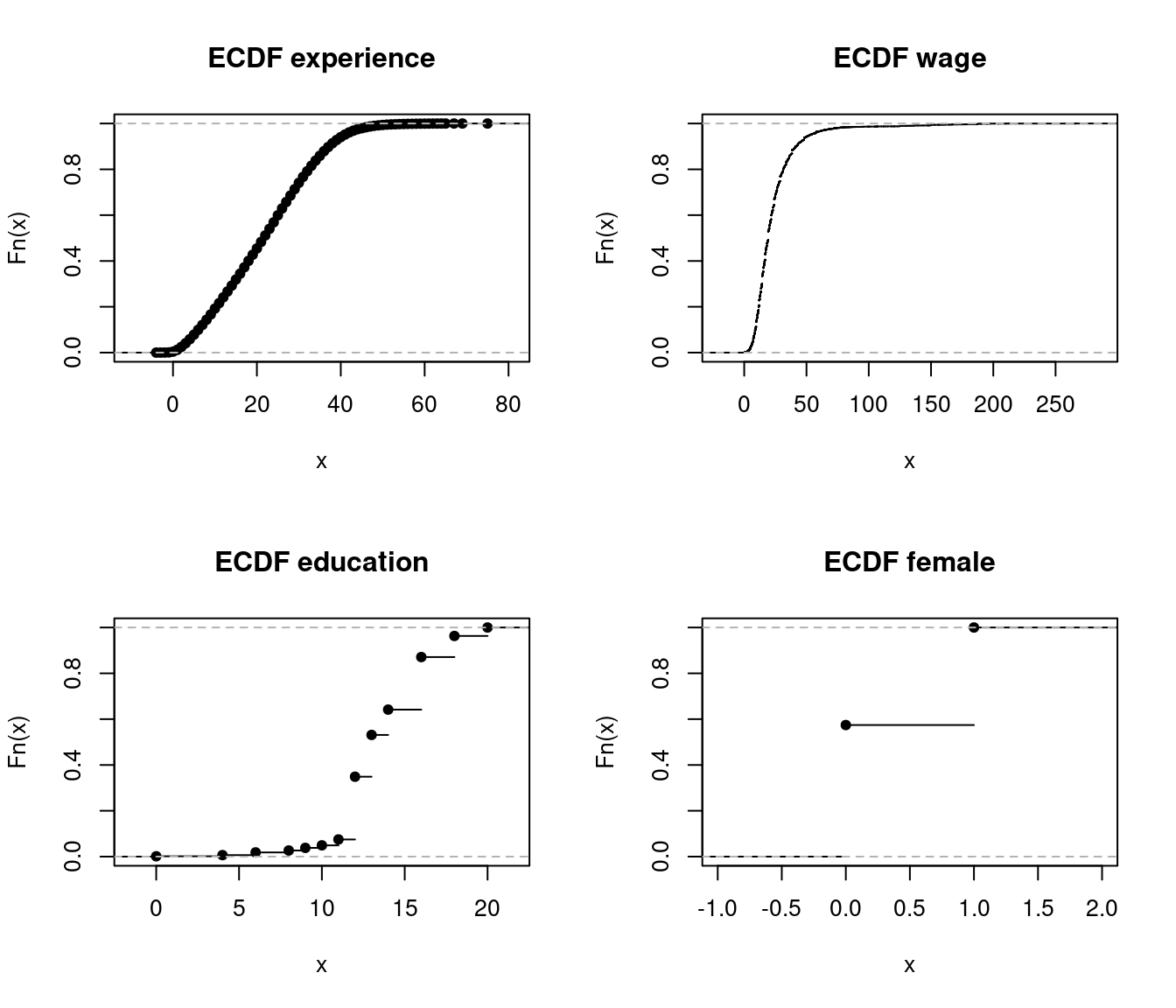
A variable is discrete if it has a countable number of possible outcomes. It is continuous if it can take any value within a range or continuum of possible outcomes. The ECDF is always a step function with steps becoming arbitrarily small for continuous distributions as n increases.
The plots show that edu and fem are discrete variables. The variable exper, although measured in years and technically discrete, has a large number of possible values, which makes it effectively “almost” continuous. On the other hand, the variable wage is clearly continuous, as it can take on a wide range of values.
2.2 Histogram
Histograms offer a more intuitive visual representation of the sample distribution compared to the ECDF. A histogram divides the data range into B bins each of equal width h and counts the number of observations n_j within each bin. The height of the histogram at a in the j-th bin is \widehat f(a) = \frac{n_j}{nh}. The histogram is the plot of these heights, displayed as rectangles, with their area normalized so that the total area equals 1.
par(mfrow = c(2,2))
hist(exper, probability = TRUE)
hist(wage, probability = TRUE)
hist(edu, probability = TRUE)
hist(fem, probability = TRUE)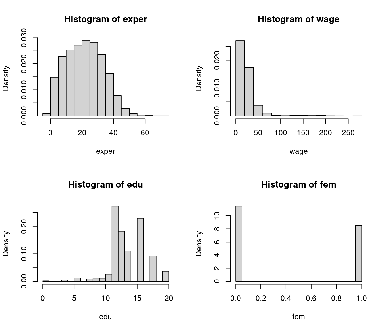
Running hist(wage, probability=TRUE) automatically selects a suitable number of bins B. Note that hist(wage) will plot absolute frequencies instead of relative ones. The shape of a histogram depends on the choice of B. You can experiment with different values using the breaks option:
2.3 Empirical quantiles
Another way of characterizing the sample distribution is to use empirical quantiles.
Median
The median is a central value that splits the distribution into two equal parts. The empirical median of a sorted dataset is found at the point where the ECDF reaches 0.5. For an even-sized dataset, the median is the average of the two central observations:
\widehat{med} = \begin{cases} Y_{(\frac{n+1}{2})} & \text{if} \ n \ \text{is odd} \\ \frac{1}{2} \big( Y_{(\frac{n}{2})} + Y_{(\frac{n}{2}+1)} \big) & \text{if} \ n \ \text{is even} \end{cases} The median corresponds to the 0.5-quantile of the distribution.
Quantile
The empirical p-quantile \widehat q_p is a value at which p percent of the data falls below it. It is found at the point where the ECDF reaches p.
Since the ECDF is flat between its jumps, the empirical p-quantile may not be unique. It can be computed as the linear interpolation at h=(n-1)p+1 between Y_{(\lfloor h \rfloor)} and Y_{(\lceil h \rceil)}: \widehat q_p = Y_{(\lfloor h \rfloor)} + (h - \lfloor h \rfloor) (Y_{(\lceil h \rceil)} - Y_{(\lfloor h \rfloor)}). Note that \lfloor h \rfloor and \lceil h \rceil denotes rounding down and rounding up to the next integer. This interpolation scheme is standard in R, although multiple approaches exist to define empirical quantiles (see here).
To calculate the 0.05 quantile, the median and the 0.95 quantile of the data, we can use the following command:
Let’s plot all quantiles as a function on a fine grid of probabilities between 0 and 1:
par(mfrow = c(2,2))
plot(probs, q.exper, type="l")
plot(probs, q.wage, type="l")
plot(probs, q.edu, type="l")
plot(probs, q.fem, type="l")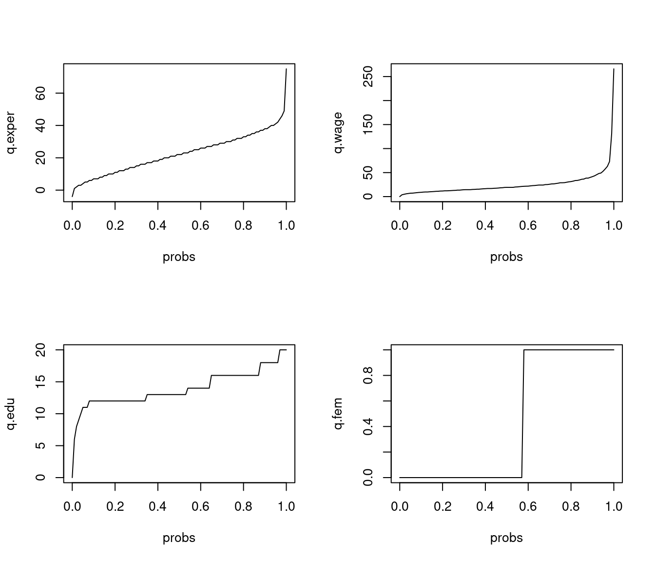
Check that these are indeed the correct quantiles using the ECDF plots from above.
2.4 Empirical moments
Many stylized features and characteristics of a sample distribution can be computed from sample moments.
2.4.1 Sample moments
The r-th sample moment about the origin (also called the raw moment) is defined as \overline{Y^r} = \frac{1}{n} \sum_{i=1}^n Y_i^r.
For example, the first sample moment (r=1) is the sample mean (arithmetic mean): \overline Y = \frac{1}{n} \sum_{i=1}^n Y_i. The sample mean is the most common measure of central tendency.
To compute the sample mean of a vector Y in R, use mean(Y) or alternatively sum(Y)/length(Y). The r-th sample moment can be calculated with mean(Y^r).
2.4.2 Central sample moments
The r-th central sample moment is the average of the r-th powers of the deviations from the sample mean: \frac{1}{n} \sum_{i=1}^n (Y_i - \overline Y)^r For example, the second central moment (r=2) is the sample variance: \widehat \sigma_Y^2 = \frac{1}{n} \sum_{i=1}^n (Y_i - \overline Y)^2 = \overline{Y^2} - \overline Y^2. The sample variance measures the spread or dispersion of the data around the sample mean.
The sample standard deviation, the square root of the sample variance: \widehat \sigma_Y = \sqrt{\widehat \sigma_Y^2} = \sqrt{\frac{1}{n} \sum_{i=1}^n (Y_i - \overline Y)^2} = \sqrt{\overline{Y^2} - \overline Y^2} It quantifies the typical deviation of data points from the sample mean in the original units of measurement.
2.4.3 Degree of freedom corrections
When computing the sample mean \overline Y, we have n degrees of freedom because each data point Y_i can vary freely. However, when calculating the deviations (Y_i - \overline Y), these deviations are subject to the constraint: \sum_{i=1}^n (Y_i - \overline{Y}) = 0. This means that the deviations are not all free to vary; they are connected by this equation. Knowing the first n-1 of the deviations determines the last one: (Y_n - \overline Y) = - \sum_{i=1}^{n-1} (Y_i - \overline Y). Therefore, only n-1 deviations can vary freely, which results in n-1 degrees of freedom for the sample variance.
Because \sum_{i=1}^{n} (Y_i - \overline Y)^2 effectively contains only n-1 freely varying summands, it is common to account for this fact. The adjusted sample variance uses n−1 in the denominator: s_Y^2 = \frac{1}{n-1} \sum_{i=1}^n (Y_i - \overline Y)^2. The adjusted sample variance relates to the unadjusted sample variance as: s_Y^2 = \frac{n}{n-1} \widehat \sigma_Y^2. The adjusted sample standard deviation is: s_Y = \sqrt{\frac{1}{n-1} \sum_{i=1}^n (Y_i - \overline Y)^2} = \sqrt{\frac{n}{n-1}} \widehat \sigma_Y.
To compute the sample variance and sample standard deviaion of a vector Y in R, use mean(Y^2)-mean(Y)^2 and sqrt(mean(Y^2)-mean(Y)^2), respectively. The built-in functions var(Y) and sd(Y) compute their adjusted versions.
2.4.4 Standardized sample moments
The r-th standardized sample moment is the central moment normalized by the sample standard deviation raised to the power of r. It is defined as: \frac{1}{n} \sum_{i=1}^n \bigg(\frac{Y_i - \overline Y}{\widehat \sigma_Y}\bigg)^r
Skewness
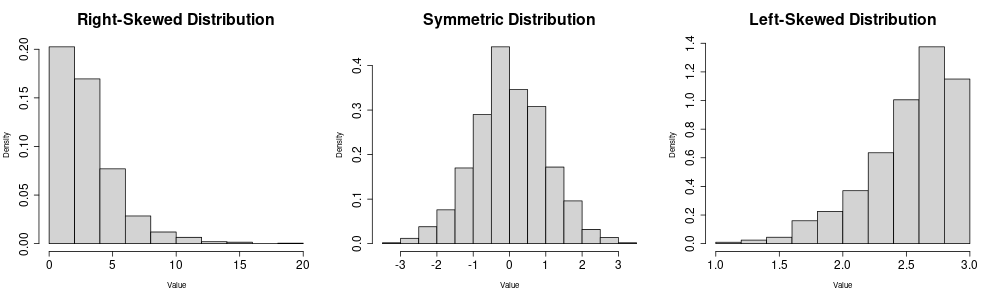
For example, the third standardized sample moment (r=3) is the sample skewness: \widehat{skew} = \frac{1}{n \widehat \sigma_Y^3} \sum_{i=1}^n (Y_i - \overline Y)^3. The skewness is a measure of asymmetry around the mean. A non-zero skewness indicates an asymmetric distribution, with positive values indicating a right tail and negative values a left tail.
To compute the sample skewness in R, use:
For convenience, you can use the skewness(Y) function from the moments package, which performs the same calculation.
[1] 0.1862605 4.3201570 -0.2253251 0.3004446Wages are right-skewed because a few very rich individuals earn much more than the many with low to medium incomes. The other variables do not indicate any pronounced skewness.
Kurtosis
The sample kurtosis is the fourth standardized sample moment (r=4): \widehat{kurt} = \frac{1}{n \widehat \sigma_Y^4} \sum_{i=1}^n (Y_i - \overline Y)^4.
Kurtosis measures the “tailedness” or heaviness of the tails of a distribution and can indicate the presence of extreme outliers. The reference value is 3, which corresponds to the kurtosis of a normal distribution (we will discuss this later in detail). Values greater than 3 suggest heavier tails, while values less than 3 indicate lighter tails.
To compute the sample kurtosis in R, use:
For convenience, you can use the kurtosis(Y) function from the moments package, which performs the same calculation.
[1] 2.374758 30.370331 4.498264 1.090267The variable wage exhibits heavy tails due to a few super-rich outliers in the sample. In contrast, fem has light tails because there are approximately equal numbers of women and men.
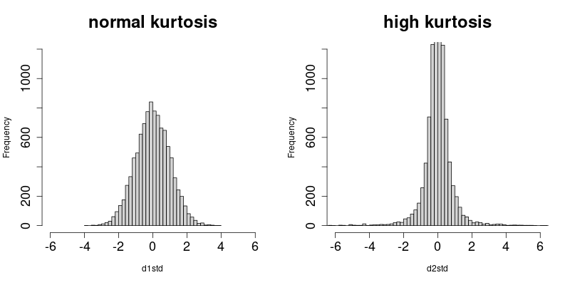
The plots display histograms of two standardized datasets (both have a sample mean of 0 and a sample variance of 1). The left dataset has a normal sample kurtosis (around 3), while the right dataset has a high sample kurtosis with heavier tails.
The plot shows histrograms of two standardized univariate datasets (i.e., their sample mean is 0 and their sample variance is 1). The dataset from the left plot has a normal sample kurtosis (around 3) and the dataset from the right plot has a high sample kurtosis with more obervarions in the tails.
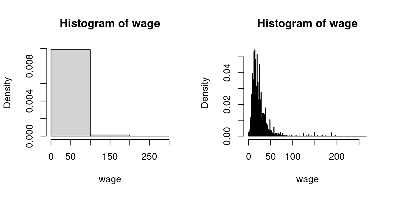
Right-skewed, heavy-tailed variables are common in real-world datasets, such as income levels, wealth accumulation, property values, insurance claims, and social media follower counts. A common transformation to reduce skewness and kurtosis in data is to use the natural logarithm:
par(mfrow = c(1,2))
hist(wage, probability = TRUE)
hist(log(wage), probability = TRUE, xlim = c(-3, 6))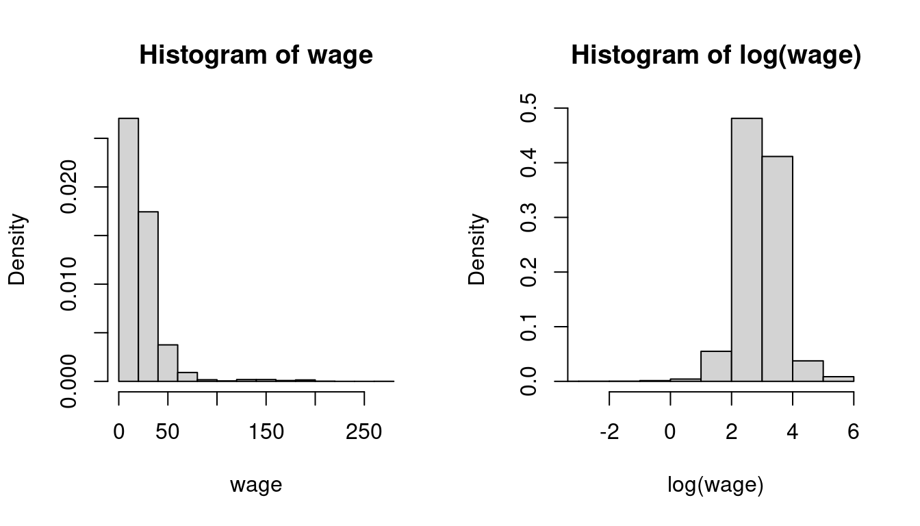
In econometrics, statistics, and many programming languages including R, \log(\cdot) is commonly used to denote the natural logarithm.
2.5 Sample covariance
Consider a multivariate dataset \boldsymbol X_1, \ldots, \boldsymbol X_n, such as the following subset of the cps dataset:
dat = data.frame(wage, edu, fem)Sample mean vector
The sample mean vector \overline{\boldsymbol X} contains the sample means of the k variables and is defined as \overline{\boldsymbol X} = \frac{1}{n} \sum_{i=1}^n \boldsymbol X_i.
colMeans(dat) wage edu fem
23.9026619 13.9246187 0.4257223 Sample covariance matrix
The sample covariance matrix \widehat{\Sigma} is the k \times k matrix given by \widehat{\Sigma} = \frac{1}{n} \sum_{i=1}^n (\boldsymbol X_i - \overline{\boldsymbol X})(\boldsymbol X_i - \overline{\boldsymbol X})'. Its elements \widehat \sigma_{h,l} represent the pairwise sample covariance between variables h and l: \widehat \sigma_{h,l} = \frac{1}{n} \sum_{i=1}^n (X_{ih} - \overline{X_h})(X_{il} - \overline{X_l}), \quad \overline{X_h} = \frac{1}{n} \sum_{i=1}^n X_{ih}.
The adjusted sample covariance matrix S is defined as S = \frac{1}{n-1} \sum_{i=1}^n (\boldsymbol X_i - \overline{\boldsymbol X})(\boldsymbol X_i - \overline{\boldsymbol X})' Its elements s_{h,l} are the adjusted sample covariances, with main diagonal elements s_{h}^2 = s_{h,h} being the adjusted sample variances: s_{h,l} = \frac{1}{n-1} \sum_{i=1}^n (X_{ih} - \overline{X_h})(X_{il} - \overline{X_l}).
cov(dat) wage edu fem
wage 428.948332 21.82614057 -1.66314777
edu 21.826141 7.53198925 0.06037303
fem -1.663148 0.06037303 0.24448764Sample correlation matrix
The sample correlation coefficient between the variables h and l is the standardized sample covariance: c_{h,l} = \frac{s_{h,l}}{s_h s_l} = \frac{\sum_{i=1}^n (X_{ih} - \overline{X_h})(X_{il} - \overline{X_l})}{\sqrt{\sum_{i=1}^n (X_{ih} - \overline{X_h})^2}\sqrt{\sum_{i=1}^n (X_{il} - \overline{X_l})^2}} = \frac{\widehat \sigma_{h,l}}{\widehat \sigma_h \widehat \sigma_l}. These coefficients form the sample correlation matrix C, expressed as:
C = D^{-1} S D^{-1}, where D is the diagonal matrix of adjusted sample standard deviations: D = diag(s_1, \ldots, s_k) = \begin{pmatrix} s_1 & 0 & \ldots & 0 \\ 0 & s_2 & \ldots & 0 \\ \vdots & & \ddots & \vdots \\ 0 & 0 & \ldots & s_k \end{pmatrix} The matrices \widehat{\Sigma}, S, and C are symmetric.
cor(dat) wage edu fem
wage 1.0000000 0.38398973 -0.16240519
edu 0.3839897 1.00000000 0.04448972
fem -0.1624052 0.04448972 1.00000000We find a strong positive correlation between wage and edu, a substantial negative correlation between wage and fem, and a negligible correlation between edu and fem.