(Intercept)   education      female
-14.081788 2.958174 -7.533067 10 Confidence intervals
10.1 Estimation uncertainty
An estimator provides an approximation of an unknown population parameter as a single real number or vector, which we call a point estimate. For instance, when we estimate the linear relationship between wage, education, and gender using an OLS, we obtain a specific set of coefficients:
However, the point estimate \widehat \beta_j alone does not reflect how close or far the estimate might be from the true population parameter \beta_j. It doesn’t capture estimation uncertainty. This inherent uncertainty arises because point estimates are based on a finite sample, which may vary from sample to sample.
Larger samples tend to give more accurate OLS estimates as OLS is unbiased and consistent under assumptions (A1)–(A4). However, we work with fixed, finite samples in practice.
Confidence intervals address this limitation by providing a range of values likely to contain the true population parameter. By constructing an interval around our point estimate that contains the true parameter with a specified probability (e.g., 95% confidence level), we can express the uncertainty more clearly.
In this section, we will introduce interval estimates, commonly referred to as confidence intervals. To construct a confidence interval for an OLS coefficient \widehat{\beta}_j, we need two components: a standard error (an estimate of the standard deviation of the estimator) and information about the distribution of \widehat{\beta}_j.
10.2 Gaussian distribution
The Gaussian distribution, also known as the normal distribution, is a fundamental concept in statistics. We often use these terms interchangeably: a random variable Z is said to follow a Gaussian or normal distribution if it has the following probability density function (PDF) with a given mean \mu and variance \sigma^2: f(u) = \frac{1}{\sqrt{2 \pi \sigma^2}} \exp\Big(-\frac{(u-\mu)^2}{2 \sigma^2}\Big). Formally, we denote this as Z \sim \mathcal N(\mu, \sigma^2), meaning that Z is normally distributed with mean \mu and variance \sigma^2.
- Mean: E[Z] = \mu
- Variance: Var(Z) = \sigma^2
- Skewness: skew(Z) = 0
- Kurtosis: kurt(Z) = 3
par(mfrow=c(1,2), bty="n", lwd=1)
x = seq(-5,9,0.01) # define grid for x-axis for the plot
plot(x, dnorm(x, mean = 2, sd = sqrt(2)), type="l", main="PDF of N(2,2)", ylab="", xlab="")
plot(x, pnorm(x, mean = 2, sd = sqrt(2)), type="l", main="CDF of N(2,2)", ylab="", xlab="")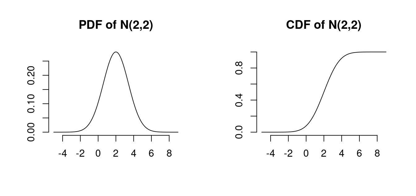
Use the R functions dnorm to calculate normal PDF values and pnorm for normal CDF values.
The Gaussian distribution with mean 0 and variance 1 is called the standard normal distribution. It has the PDF \phi(u) = \frac{1}{\sqrt{2 \pi}} \exp\Big(-\frac{u^2}{2}\Big) and CDF \Phi(a) = \int_{-\infty}^a \phi(u) \ \text{d}u. \mathcal N(0,1) is symmetric around zero: \phi(u) = \phi(-u), \quad \Phi(a) = 1 - \Phi(-a)
Standardizing: If Z \sim \mathcal N(\mu, \sigma^2), then \frac{Z-\mu}{\sigma} \sim \mathcal N(0,1), and the CDF of Z is \Phi((Z-\mu)/\sigma).
Linear combinations of normally distributed variables are normal: If Y_1, \ldots, Y_n are normally distributed and c_1, \ldots, c_n \in \mathbb R, then \sum_{j=1}^n c_j Y_j is normally distributed.
10.2.1 Multivariate Gaussian distribution
Let Z_1, \ldots, Z_k be independent \mathcal N(0,1) random variables. Then, the k-vector \boldsymbol Z = (Z_1, \ldots, Z_k)' has the multivariate standard normal distribution, written \boldsymbol Z \sim \mathcal N(\boldsymbol 0, \boldsymbol I_k). Its joint density is f(\boldsymbol u) = \frac{1}{(2 \pi)^{k/2}} \exp\left( - \frac{\boldsymbol u'\boldsymbol u}{2} \right).
If \boldsymbol Z \sim \mathcal N(\boldsymbol 0, \boldsymbol I_k) and \boldsymbol Z^* = \boldsymbol \mu + \boldsymbol B \boldsymbol Z for a q \times 1 vector \boldsymbol \mu and a q \times k matrix \boldsymbol B, then \boldsymbol Z^* has a multivariate normal distribution with mean vector \boldsymbol \mu and covariance matrix \boldsymbol \Sigma = \boldsymbol B \boldsymbol B', written \boldsymbol Z^* \sim \mathcal N(\boldsymbol \mu, \boldsymbol \Sigma). The k-variate PDF of \boldsymbol Z^* is f(\boldsymbol u) = \frac{1}{(2 \pi)^{k/2} (\det(\boldsymbol \Sigma))^{1/2} } \exp\Big(- \frac{1}{2}(\boldsymbol u-\boldsymbol \mu)'\boldsymbol \Sigma^{-1} (\boldsymbol u-\boldsymbol\mu) \Big).
The mean vector and covariance matrix are E[\boldsymbol Z^*] = \boldsymbol \mu, \quad Var(\boldsymbol Z^*) = \boldsymbol \Sigma.
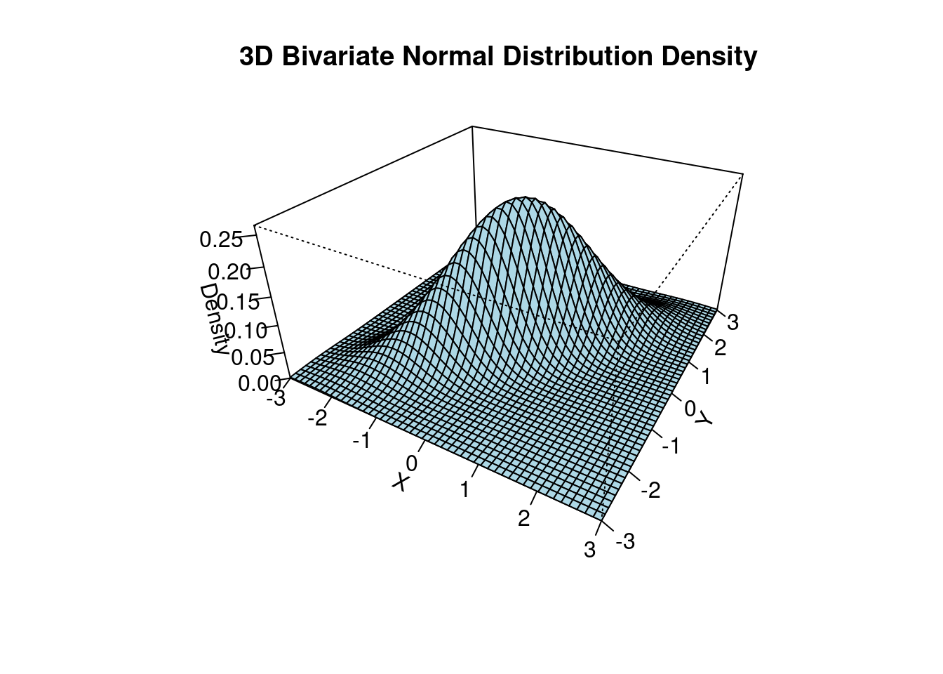
The 3d plot shows the bivariate normal PDF with parameters \boldsymbol \mu = \begin{pmatrix} 0 \\ 0 \end{pmatrix}, \quad \boldsymbol \Sigma = \begin{pmatrix} 1 & 0.8 \\ 0.8 & 1 \end{pmatrix}.
10.2.2 Chi-squared distribution
Let Z_1, \ldots, Z_m be independent \mathcal N(0,1) random variables. Then, the random variable Y = \sum_{i=1}^m Z_i^2 is chi-squared distributed with parameter m, written Y \sim \chi^2_{m}.
The parameter m is called the degrees of freedom.
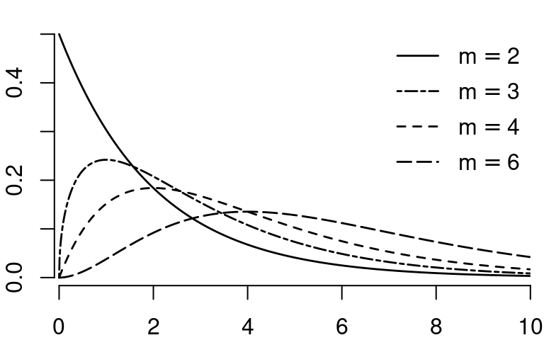
- Mean: E[Y] = m
- Variance: Var(Y) = 2m
- Skewness: skew(Y) = \sqrt{8/m}
- Kurtosis: kurt(Y) = 3+12/m
10.2.3 Student t-distribution
If Z \sim \mathcal N(0,1) and Q \sim \chi^2_{m}, and Z and Q are independent, then Y = \frac{Z}{\sqrt{Q/m}} is t-distributed with parameter m degrees of freedom, written Y \sim t_m.
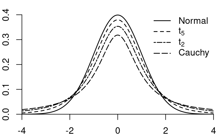
The t-distribution with m=1 is also called Cauchy distribution. The t-distributions with 1, 2, 3, and 4 degrees of freedom are heavy-tailed distributions. If m \to \infty then t_m \to \mathcal N(0,1)
- Mean: E[Y] = 0 if m \geq 2
- Variance: Var(Y) = \frac{m}{m-2} if m \geq 3
- Skewness: skew(Y) = 0 if m \geq 4
- Kurtosis: kurt(Y) = 3+6/(m-4) if m \geq 5
The kurtosis is infinite for m \leq 4, the skewness is undefined for m \leq 3, the variance is infinite for m \leq 2, and the mean is undefined for m=1.
10.3 Classical Gaussian regression model
Let’s revisit the linear regression model: Y_i = \boldsymbol X_i'\boldsymbol \beta + u_i, \quad i=1, \ldots, n. \tag{10.1} Under assumptions (A1)–(A4), the distributional restrictions on the error term are relatively mild:
The error terms are i.i.d. but can have different conditional variances depending on the values of the regressors (heteroskedasticity): Var(u_i | \boldsymbol X_i) = \sigma^2(\boldsymbol X_i) = \sigma_i^2. For example, in a regression of
wageonfemale, the error variances for women may differ from those for men.The error term can follow any distribution, provided that the fourth moment (the kurtosis) is finite. This excludes heavy-tailed distributions.
In standard introductory textbooks, two additional assumptions are often made to further restrict the properties mentioned above. It is beneficial to first study the estimation uncertainty under this simplified setting.
Classical Gaussian regression model
In addition to the linear regression model in Equation 10.1 with assumptions (A1)–(A4), we introduce two more assumptions:
(A5) Homoskedasticity: The error terms have constant variance across all observations, i.e., Var(u_i | \boldsymbol X_i) = \sigma_i^2 = \sigma^2 \quad \text{for all} \ i=1, \ldots, n.
(A6) Normality: The error terms are normally distributed conditional on the regressors, i.e., u_i | \boldsymbol X_i \sim \mathcal N(0, \sigma_i^2).
(A5)-(A6) combined can be expressed as: u_i | \boldsymbol X_i \sim \mathcal N(0, \sigma^2) \quad \text{for all} \ i=1, \ldots, n.
The notation u_i | \boldsymbol X_i \sim \mathcal N(0, \sigma^2) means that the conditional distribution of u_i conditional on \boldsymbol X_i is N(0, \sigma^2). The PDF of u_i | \boldsymbol X_i is f(u) = \frac{1}{\sqrt{2 \pi \sigma^2}} \exp\Big(-\frac{u^2}{2 \sigma^2}\Big).
Distribution of the OLS coefficients
Conditional on \boldsymbol X, the OLS coefficient vector is a linear combination of the error term: \begin{align*} \widehat{\boldsymbol \beta} &= (\boldsymbol X'\boldsymbol X)^{-1} \boldsymbol X' \boldsymbol Y \\ &= \boldsymbol \beta + (\boldsymbol X'\boldsymbol X)^{-1} \boldsymbol X' \boldsymbol u. \end{align*} Consequently, under (A6), the OLS estimator follows a k-variate normal distribution, conditionally on \boldsymbol X.
Recall that the mean is E[\widehat{\boldsymbol \beta}|\boldsymbol X] = \boldsymbol \beta and the covariance matrix is Var(\widehat{\boldsymbol \beta}|\boldsymbol X) = (\boldsymbol X'\boldsymbol X)^{-1} \boldsymbol X' \boldsymbol D \boldsymbol X (\boldsymbol X'\boldsymbol X)^{-1}. Under homoskedasticity (A5), we have \boldsymbol D = \sigma^2 \boldsymbol I_n, so the covariance matrix simplifies to Var(\widehat{\boldsymbol \beta}|\boldsymbol X) = \sigma^2 (\boldsymbol X'\boldsymbol X)^{-1}. Therefore, \widehat{\boldsymbol \beta}|\boldsymbol X \sim \mathcal N(\boldsymbol \beta, \sigma^2 (\boldsymbol X'\boldsymbol X)^{-1}). The variance of the j-th OLS coefficient is Var(\widehat{\beta}_j|\boldsymbol X) = \sigma^2 [(\boldsymbol X'\boldsymbol X)^{-1}]_{jj}, where [(\boldsymbol X'\boldsymbol X)^{-1}]_{jj} indicates the j-th diagonal element of the matrix (\boldsymbol X'\boldsymbol X)^{-1}. The standard deviation is: sd(\widehat \beta_j|\boldsymbol X) = \sqrt{\sigma^2 [(\boldsymbol X'\boldsymbol X)^{-1}]_{jj}}. Therefore, the standardized OLS coefficient has a standard normal distribution: Z_j := \frac{\widehat \beta_j - \beta_j}{sd(\widehat \beta_j|\boldsymbol X)} \sim \mathcal N(0,1). \tag{10.2}
10.4 Confidence interval: known variance
One of the most common methods of incorporating estimation uncertainty into estimation results is through interval estimates, often referred to as confidence intervals.
A confidence interval is a range of values that is likely to contain the true population parameter with a specified confidence level or coverage probability, often expressed as a percentage (e.g., 95%). For example, a 95% confidence interval suggests that, across many repeated samples, approximately 95% of the intervals constructed from those samples would contain the true population parameter.
A symmetric confidence interval for \beta_j with confidence level 1-\alpha is an interval I_{1-\alpha} = [\widehat \beta_j - c_{1-\alpha}; \widehat \beta_j + c_{1-\alpha}] with the property that P(\beta_j \in I_{1-\alpha}) = 1-\alpha. \tag{10.3} Common coverage probabilities are 0.95, 0.99, and 0.90.
Note that I_{1-\alpha} is random and \beta_j is fixed but unknown. Therefore, the coverage probability is the probability that this random interval I_{1-\alpha} contains the true parameter.
A more precise interpretation of a confidence interval is:
If we were to repeat the sampling process and construct confidence intervals for each sample, 1-\alpha of those intervals would contain the true population parameter.
It is essential to understand that the confidence interval reflects the reliability of the method, not the probability of the true parameter falling within a particular interval. The interval itself is random – it varies with each sample – but the population parameter is fixed and unknown.
Thus, it is incorrect to interpret a specific confidence interval as having a 95% probability of containing the true value. Instead, the correct interpretation is that the method used to calculate the interval has a 95% success rate across many samples.
The width of the interval
The OLS coefficient \widehat \beta_j is in the center of I_{1-\alpha}. Let’s solve for c_{1-\alpha} to get the width of the confidence interval.
The event \{\beta_j \in I_{1-\alpha}\} can be rearranged as \begin{align*} &\phantom{\Leftrightarrow} \quad \beta_j \in I_{1-\alpha} \\ &\Leftrightarrow \quad \widehat \beta_j - c_{1-\alpha} \leq \beta_j \leq \widehat \beta_j + c_{1-\alpha} \\ &\Leftrightarrow \quad - c_{1-\alpha} \leq \beta_j - \widehat \beta_j \leq c_{1-\alpha} \\ &\Leftrightarrow \quad c_{1-\alpha} \geq \widehat \beta_j - \beta_j \geq - c_{1-\alpha} \\ &\Leftrightarrow \quad \frac{c_{1-\alpha}}{sd(\widehat \beta_j|\boldsymbol X)} \geq Z_j \geq - \frac{c_{1-\alpha}}{sd(\widehat \beta_j|\boldsymbol X)} \end{align*} with Z_j defined in Equation 10.2. Hence, Equation 10.3 becomes P\bigg(\frac{- c_{1-\alpha}}{sd(\widehat \beta_j|\boldsymbol X)} \leq Z_j \leq \frac{c_{1-\alpha}}{sd(\widehat \beta_j|\boldsymbol X)}\bigg) = 1-\alpha. \tag{10.4} Since Z_j is standard normal by Equation 10.2, we have \begin{align*} &P\bigg(\frac{- c_{1-\alpha}}{sd(\widehat \beta_j|\boldsymbol X)} \leq Z_j \leq \frac{c_{1-\alpha}}{sd(\widehat \beta_j|\boldsymbol X)}\bigg) \\ &= \Phi\bigg( \frac{c_{1-\alpha}}{sd(\widehat \beta_j|\boldsymbol X)} \bigg) - \Phi\bigg( \frac{-c_{1-\alpha}}{sd(\widehat \beta_j|\boldsymbol X)} \bigg) \\ &= \Phi\bigg( \frac{c_{1-\alpha}}{sd(\widehat \beta_j|\boldsymbol X)} \bigg) - \bigg( 1 - \Phi\bigg( \frac{c_{1-\alpha}}{sd(\widehat \beta_j|\boldsymbol X)} \bigg) \bigg) \\ &= 2\Phi\bigg( \frac{c_{1-\alpha}}{sd(\widehat \beta_j|\boldsymbol X)} \bigg) - 1. \end{align*} With Equation 10.4, we get 1-\alpha = 2\Phi\bigg( \frac{c_{1-\alpha}}{sd(\widehat \beta_j|\boldsymbol X)} \bigg) - 1. Let’s add 1 and divide by 2: 1- \frac{\alpha}{2} = \Phi\bigg( \frac{c_{1-\alpha}}{sd(\widehat \beta_j|\boldsymbol X)} \bigg), \tag{10.5} where (2-\alpha)/2 = 1-\alpha/2.
The value z_{(p)} is the p-quantile of \mathcal N(0,1) if \Phi(z_{(p)}) = p. We write \Phi^{-1}(p) = z_{(p)}, where the quantile function \Phi^{-1} is the inverse function of the CDF \Phi with \Phi(\Phi^{-1}(p)) = p and \Phi^{-1}(\Phi^{-1}(z)) = z.
Then, applying the quantile function \Phi^{-1} to Equation 10.5 gives: \begin{align*} &\Leftrightarrow& \quad \Phi^{-1}\bigg(1 - \frac{\alpha}{2} \bigg) &= \frac{c_{1-\alpha}}{sd(\widehat \beta_j|\boldsymbol X)} \\ &\Leftrightarrow& \quad z_{(1-\frac{\alpha}{2})} &= \frac{c_{1-\alpha}}{sd(\widehat \beta_j|\boldsymbol X)} \\ &\Leftrightarrow& \quad z_{(1-\frac{\alpha}{2})} \cdot sd(\widehat \beta_j|\boldsymbol X) &= c_{1-\alpha}, \end{align*} where z_{(1-\frac{\alpha}{2})} is the 1-\alpha/2-quantile of \mathcal N(0,1). The solution for the confidence interval is: I_{1-\alpha} = \Big[\widehat \beta_j - z_{(1-\frac{\alpha}{2})} \cdot sd(\widehat \beta_j|\boldsymbol X); \ \widehat \beta_j + z_{(1-\frac{\alpha}{2})} \cdot sd(\widehat \beta_j|\boldsymbol X)\Big].
Standard normal quantiles can be obtained using the R command qnorm or by using statistical tables:
| 0.9 | 0.95 | 0.975 | 0.99 | 0.995 |
| 1.28 | 1.64 | 1.96 | 2.33 | 2.58 |
Therefore, 90%, 95%, and 99% confidence intervals for \beta_j are given by \begin{align*} I_{0.9} &= [\widehat \beta_j - 1.64 \cdot sd(\widehat \beta_j|\boldsymbol X); \ \widehat \beta_j + 1.64 \cdot sd(\widehat \beta_j|\boldsymbol X)] \\ I_{0.95} &= [\widehat \beta_j - 1.96 \cdot sd(\widehat \beta_j|\boldsymbol X); \ \widehat \beta_j + 1.96 \cdot sd(\widehat \beta_j|\boldsymbol X)] \\ I_{0.99} &= [\widehat \beta_j - 2.58 \cdot sd(\widehat \beta_j|\boldsymbol X); \ \widehat \beta_j + 2.58 \cdot sd(\widehat \beta_j|\boldsymbol X)] \end{align*}
With probability \alpha, the interval does not cover the true parameter. The smaller we choose \alpha, the more confident we can be that the interval covers the true parameter, but the larger the interval becomes. If we set \alpha = 0, the interval would be infinite, providing no useful information.
A certain amount of uncertainty always remains, but we can control it by choosing an appropriate value for \alpha that balances our desired level of confidence with the precision of the estimate. This is why the coverage probability (1-\alpha) is also called the confidence level.
Note that this interval is infeasible in practice because the conditional standard deviation is unknown: sd(\widehat \beta_j|\boldsymbol X) = \sqrt{\sigma^2 [(\boldsymbol X'\boldsymbol X)^{-1}]_{jj}}. It requires knowledge about the true error variance Var(u_i|\boldsymbol X) = \sigma^2.
10.5 Classical standard errors
A standard error se(\widehat \beta_j) for an estimator \widehat \beta_j is an estimator of the standard deviation of the distribution of \widehat \beta_j.
We say that the standard error is consistent if \frac{se(\widehat \beta_j)}{sd(\widehat \beta_j | \boldsymbol X)} \overset{p}{\to} 1. \tag{10.6}
This property ensures that, in practice, we can replace the unknown standard deviation with the standard error in confidence intervals.
Under the classical Gaussian regression model, we have sd(\widehat \beta_j|\boldsymbol X) = \sqrt{\sigma^2 [(\boldsymbol X'\boldsymbol X)^{-1}]_{jj}}. Therefore, it is natural to replace the population error variance \sigma^2 by the adjusted sample variance of the residuals: s_{\widehat u}^2 = \frac{1}{n-k} \sum_{i=1}^n \widehat u_i^2 = SER^2. The classical homoskedastic standard errors are: se_{hom}(\widehat \beta_j) = \sqrt{s_{\widehat u}^2 [(\boldsymbol X'\boldsymbol X)^{-1}]_{jj}}. The classical homoskedastic covariance matrix estimator for Var(\widehat{\boldsymbol \beta}|\boldsymbol X) is \widehat{\boldsymbol V}_{hom} = s_{\widehat u}^2 (\boldsymbol X'\boldsymbol X)^{-1}
fit = lm(wage ~ education + female, data = cps)
## classical homoskedastic covariance matrix estimator:
vcov(fit)
(Intercept) education female
(Intercept) 0.18825476 -0.0127486354 -0.0089269796
education -0.01274864 0.0009225111 -0.0002278021
female -0.00892698 -0.0002278021 0.0284200217The classical standard errors are the square roots of the diagonal elements of this matrix:
(Intercept)   education      female
 0.43388334  0.03037287  0.16858239
These standard errors are also displayed in the second column of a regression output:
summary(fit)
Call:
lm(formula = wage ~ education + female, data = cps)

Residuals:
    Min      1Q  Median      3Q     Max
-45.071  -9.035  -2.973   4.472 244.491

Coefficients:
             Estimate Std. Error t value Pr(>|t|)
(Intercept) -14.08179    0.43388  -32.45   <2e-16 ***
education     2.95817    0.03037   97.39   <2e-16 ***
female       -7.53307    0.16858  -44.69   <2e-16 ***
---
Signif. codes:  0 '***' 0.001 '**' 0.01 '*' 0.05 '.' 0.1 ' ' 1

Residual standard error: 18.76 on 50739 degrees of freedom
Multiple R-squared:  0.1797,    Adjusted R-squared:  0.1797
F-statistic:  5559 on 2 and 50739 DF,  p-value: < 2.2e-16
Because s_{\widehat u}^2/\sigma^2 \overset{p}{\rightarrow} 1, property Equation 10.6 is satisfied and se_{hom}(\widehat \beta_j) is a consistent standard error under homoskedasticity.
Note that the main result we used to derive the confidence interval is that the standardized OLS coefficient is standard normal: Z_j := \frac{\widehat \beta_j - \beta_j}{sd(\widehat \beta_j|\boldsymbol X)} \sim \mathcal N(0,1). If we replace the unknown standard deviation sd(\widehat \beta_j|\boldsymbol X) with the standard error se_{hom}(\widehat \beta_j), the distribution changes.
The OLS estimator standardized with the standard error is called t-statistic: T_j = \frac{\widehat \beta_j - \beta_j}{se_{hom}(\widehat \beta_j)} = \frac{sd(\widehat \beta_j|\boldsymbol X)}{se_{hom}(\widehat \beta_j)} \frac{\widehat \beta_j - \beta_j}{sd(\widehat \beta_j|\boldsymbol X)} = \frac{sd(\widehat \beta_j|\boldsymbol X)}{se_{hom}(\widehat \beta_j)} Z_j. The additional factor satisfies \frac{sd(\widehat \beta_j|\boldsymbol X)}{se_{hom}(\widehat \beta_j)} = \frac{\sigma}{s_{\widehat u}} \sim \sqrt{(n-k)/\chi^2_{n-k}}, where \chi^2_{n-k} is the chi-squared distribution with n-k degrees of freedom, independent of Z_j.
Therefore, the t-statistic is t-distributed: T_j = \frac{\widehat \beta_j - \beta_j}{se_{hom}(\widehat \beta_j)} = \frac{\sigma}{s_{\widehat u}} Z_j \sim \frac{\mathcal N(0,1)}{\sqrt{\chi^2_{n-k}/(n-k)}} = t_{n-k}. \tag{10.7}
Consequently, if we replace the unknown standard deviation sd(\widehat \beta_j|\boldsymbol X) with the standard error se_{hom}(\widehat \beta_j) in the confidence interval formula, we have to replace the standard normal quantiles by t-quantiles: I_{1-\alpha}^{(hom)} = \big[\widehat \beta_j - t_{(1-\frac{\alpha}{2},n-k)} se_{hom}(\widehat \beta_j); \ \widehat \beta_j + t_{(1-\frac{\alpha}{2},n-k)} se_{hom}(\widehat \beta_j)\big] This interval is feasible and satisfies P(\beta_j \in I_{1-\alpha}^{(hom)}) = 1-\alpha under (A1)–(A6).
Click to see Student's t-distribution quantiles
| df | 0.9 | 0.95 | 0.975 | 0.99 | 0.995 |
|---|---|---|---|---|---|
| 1 | 3.08 | 6.31 | 12.71 | 31.82 | 63.66 |
| 2 | 1.89 | 2.92 | 4.30 | 6.96 | 9.92 |
| 3 | 1.64 | 2.35 | 3.18 | 4.54 | 5.84 |
| 4 | 1.53 | 2.13 | 2.78 | 3.75 | 4.60 |
| 5 | 1.48 | 2.02 | 2.57 | 3.36 | 4.03 |
| 6 | 1.44 | 1.94 | 2.45 | 3.14 | 3.71 |
| 8 | 1.40 | 1.86 | 2.31 | 2.90 | 3.36 |
| 10 | 1.37 | 1.81 | 2.23 | 2.76 | 3.17 |
| 15 | 1.34 | 1.75 | 2.13 | 2.60 | 2.95 |
| 20 | 1.33 | 1.72 | 2.09 | 2.53 | 2.85 |
| 25 | 1.32 | 1.71 | 2.06 | 2.49 | 2.79 |
| 30 | 1.31 | 1.70 | 2.04 | 2.46 | 2.75 |
| 40 | 1.30 | 1.68 | 2.02 | 2.42 | 2.70 |
| 50 | 1.30 | 1.68 | 2.01 | 2.40 | 2.68 |
| 60 | 1.30 | 1.67 | 2.00 | 2.39 | 2.66 |
| 80 | 1.29 | 1.66 | 1.99 | 2.37 | 2.64 |
| 100 | 1.29 | 1.66 | 1.98 | 2.36 | 2.63 |
| \to \infty | 1.28 | 1.64 | 1.96 | 2.33 | 2.58 |
We can use the coefci function from the AER package:
10.6 Confidence intervals: heteroskedasticity
The exact confidence interval I_{1-\alpha}^{(hom)} is only valid under the restrictive assumption of homoskedasticity (A5) and normality (A6).
For historical reasons, statistics books often treat homoskedasticity as the standard case and heteroskedasticity as a special case. However, this does not reflect empirical practice since we have to expect heteroskedastic errors in most applications. It turns out that heteroskedasticity is not a problem as long as the robust standard errors are used.
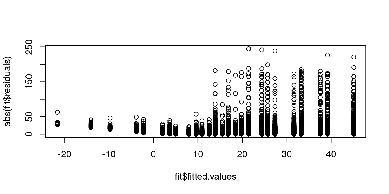
A plot of the absolute value of the residuals against the fitted values shows that individuals with predicted wages around 10 USD exhibit residuals with lower variance compared to those with higher predicted wage levels. Hence, the homoskedasticity assumption (A5) is implausible.
If (A5) does not hold, then standard deviation is
sd(\widehat \beta_j | \boldsymbol X) = \sqrt{[(\boldsymbol X'\boldsymbol X)^{-1} \boldsymbol X' \boldsymbol D \boldsymbol X (\boldsymbol X'\boldsymbol X)^{-1}]_{jj}}.
To estimate sd(\widehat \beta_j | \boldsymbol X), we will have to replace the diagonal matrix
\boldsymbol D = diag(\sigma_1^2, \ldots, \sigma_n^2)
by some sample counterpart \widehat{\boldsymbol D} = diag(\widehat \sigma_1^2, \ldots, \widehat \sigma_n^2).
Various heteroskedasticity-consistent (HC) standard errors have been proposed in the literature:
| HC type | weights |
|---|---|
| HC0 | \widehat \sigma_i^2 = \widehat u_i^2 |
| HC1 | \widehat \sigma_i^2 = \frac{n}{n-k} \widehat u_i^2 |
| HC2 | \widehat \sigma_i^2 = \frac{\widehat u_i^2}{1-h_{ii}} |
| HC3 | \widehat \sigma_i^2 = \frac{\widehat u_i^2}{(1-h_{ii})^2} |
HC0 replaces the unknown variances with squared residuals, and HC1 is a bias-corrected version of HC0. HC2 and HC3 use the leverage values h_{ii} (the diagonal entries of the influence matrix \boldsymbol P) and give less weight to influential observations.
HC1 and HC3 are the most common choices and can be written as \begin{align*} se_{hc1}(\widehat \beta_j) &= \sqrt{\Big[(\boldsymbol X' \boldsymbol X)^{-1} \Big( \frac{n}{n-k} \sum_{i=1}^n \widehat u_i^2 \boldsymbol X_i \boldsymbol X_i' \Big) (\boldsymbol X' \boldsymbol X)^{-1}\Big]_{jj}}, \\ se_{hc3}(\widehat \beta_j) &= \sqrt{\Big[(\boldsymbol X' \boldsymbol X)^{-1} \Big( \sum_{i=1}^n \frac{\widehat u_i^2}{(1-h_{ii})^2} \boldsymbol X_i \boldsymbol X_i' \Big) (\boldsymbol X' \boldsymbol X)^{-1}\Big]_{jj}}. \end{align*}
All versions perform similarly well in large samples, but HC3 performs best in small samples and is the preferred choice.
HC standard errors are also known as heteroskedasticity-robust standard errors or simply robust standard errors.
Estimators for the full covariance matrix of \widehat{\boldsymbol \beta} have the form \widehat{\boldsymbol V} = (\boldsymbol X' \boldsymbol X)^{-1} \boldsymbol X' \widehat{\boldsymbol D} \boldsymbol X (\boldsymbol X' \boldsymbol X)^{-1}. The HC3 covariance estimator can be written as \widehat{\boldsymbol V}_{hc3} = (\boldsymbol X' \boldsymbol X)^{-1} \Big( \sum_{i=1}^n \frac{\widehat u_i^2}{(1-h_{ii})^2} \boldsymbol X_i \boldsymbol X_i' \Big) (\boldsymbol X' \boldsymbol X)^{-1}.
Therefore, we can use confidence intervals of the form: I_{1-\alpha}^{(hc)} = \big[\widehat \beta_j - t_{(1-\frac{\alpha}{2},n-k)} se_{hc}(\widehat \beta_j); \ \widehat \beta_j + t_{(1-\frac{\alpha}{2},n-k)} se_{hc}(\widehat \beta_j)\big].
In contrast to Equation 10.7, the distribution of the ratio sd(\widehat \beta_j|\boldsymbol X)/se_{hc}(\widehat \beta_j) is unknown in practice, and the t-statistic is not t-distributed.
However, for large n, we have T_j^{(hc)} = \frac{\widehat \beta_j - \beta_j}{se_{hc}(\widehat \beta_j)} = \underbrace{\frac{sd(\widehat \beta_j|\boldsymbol X)}{se_{hc}(\widehat \beta_j)}}_{\overset{p}{\rightarrow} 1} \underbrace{Z_j}_{\sim \mathcal N(0,1)} which implies that \lim_{n \to \infty} P(\beta_j \in I_{1-\alpha}^{(hc)}) = 1-\alpha. \tag{10.8} Therefore I_{1-\alpha}^{(hc)} is an asymptotic confidence interval for \beta_j.
## HC3 covariance matrix estimate Vhat-hc3
vcovHC(fit)
(Intercept) education female
(Intercept) 0.25013606 -0.019590435 0.013394891
education -0.01959043 0.001609169 -0.002173848
female 0.01339489 -0.002173848 0.026131235(Intercept) education female
0.50013604 0.04011445 0.16165158 (Intercept) education female
0.50007811 0.04011017 0.16164436 coefci(fit, vcov = vcovHC, level = 0.99) 0.5 % 99.5 %
(Intercept) -15.370102 -12.793475
education 2.854842 3.061506
female -7.949469 -7.116664Robust confidence intervals can also be used and hold asymptotically under (A5). Therefore, the exact classical confidence intervals should only be used if there are very good reasons for the error terms to be homoskedastic and normally distributed.
10.7 Confidence interval with non-normal errors
Similar to the homoskedasticity assumption (A5), the normality assumption (A6) is also not satisfied in most applications. A useful diagnostic plot is the Q-Q-plot.
The Q-Q-plot is a graphical tool to help us assess if the errors are conditionally normally distributed, i.e. whether assumption (A6) is satisfied.
Let \widehat u_{(i)} be the sorted residuals (i.e. \widehat u_{(1)} \leq \ldots \leq \widehat u_{(n)}). The Q-Q-plot plots the sorted residuals \widehat u_{(i)} against the ((i-0.5)/n)-quantiles of the standard normal distribution.
If the residuals are lined well on the straight dashed line, there is indication that the distribution of the residuals is close to a normal distribution.
par(mfrow = c(1,2))
# Normally distributed response variable
plot(lm(rnorm(500) ~ 1), which = 2)
plot(fit, which=2)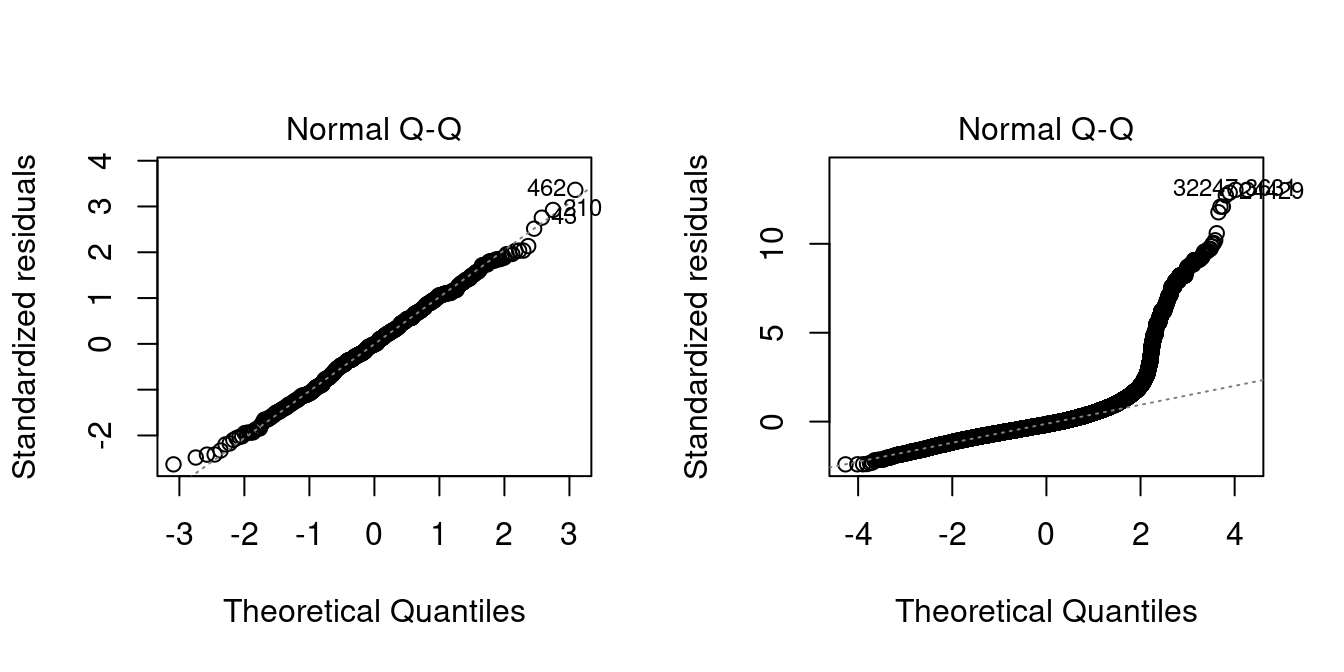
In the left plot you see the Q-Q-plot for an example with normally distributed errors. The right plot indicates that, in our regression of wage on education and female, the normality assumption is implausible.
If (A6) does not hold, then Z_j is not normally distributed, and it is unclear whether Equation 10.8 holds. However, by the central limit theorem, we still can establish that \lim_{n \to \infty} P(\beta_j \in I_{1-\alpha}^{(hc)}) = 1-\alpha. Therefore, the robust confidence interval I_{1-\alpha}^{(hc)} is asymptotically valid if (A1)–(A4) hold.
10.8 Central limit theorem
Convergence in distribution
Let \boldsymbol W_n be a sequence of k-variate random variables and let \boldsymbol V be a k-variate random variable
\boldsymbol W_n converges in distribution to \boldsymbol V, written \boldsymbol W_n \overset{d}{\rightarrow} \boldsymbol V, if \lim_{n \to \infty} P(\boldsymbol W_n \leq \boldsymbol a) = P(\boldsymbol V \leq \boldsymbol a) for all \boldsymbol a at which the CDF of \boldsymbol V is continuous.
If \boldsymbol V has the distribution \mathcal N(\boldsymbol \mu, \boldsymbol \Sigma), we write \boldsymbol W_n \overset{d}{\rightarrow} \mathcal N(\boldsymbol \mu, \boldsymbol \Sigma).
Consider for simplicity the regression on an intercept only. In this case, we have k=1 and \widehat \beta_1 = \overline Y (see the second problem set).
By the univariate central limit theorem, the centered sample mean converges to a normal distribution:
Central Limit Theorem (CLT)
Let \{Y_1, \ldots, Y_n\} be an i.i.d. sample with E[Y_i] = \mu and 0 < Var(Y_i) = \sigma^2 < \infty. Then, the sample mean satisfies \sqrt n \bigg( \frac{1}{n} \sum_{i=1}^n Y_i - \mu \bigg) \overset{d}{\longrightarrow} \mathcal N(0,\sigma^2).
Below, you will find an interactive shiny app for the central limit theorem:
The same result can be extended to k-variate random vectors.
Multivatiate Central Limit Theorem (MCLT)
If \{\boldsymbol W_1, \ldots, \boldsymbol W_n\} is an i.i.d. sample with E[\boldsymbol W_i] = \boldsymbol \mu and Var(\boldsymbol W_i) = \boldsymbol \Sigma < \infty. Then, \sqrt n \bigg( \frac{1}{n} \sum_{i=1}^n \boldsymbol W_i - \boldsymbol \mu \bigg) \overset{d}{\to} \mathcal N(\boldsymbol 0, \boldsymbol \Sigma) (see, e.g., Stock and Watson Section 19.2).
If we apply the MCLT to the random sequence \boldsymbol W_i = \boldsymbol X_i u_i with E[\boldsymbol X_i u_i] = \boldsymbol 0 and Var(\boldsymbol X_i u_i) = \boldsymbol \Omega = E[u_i^2 \boldsymbol X_i \boldsymbol X_i'], then we get \sqrt n \bigg( \frac{1}{n} \sum_{i=1}^n \boldsymbol X_i u_i \bigg) \overset{d}{\to} \mathcal N(\boldsymbol 0, \boldsymbol \Omega). Therefore, we get \sqrt n (\widehat{\boldsymbol \beta} - \boldsymbol \beta) = \sqrt n \bigg( \frac{1}{n} \sum_{i=1}^n \boldsymbol X_i \boldsymbol X_i' \bigg)^{-1} \bigg( \frac{1}{n} \sum_{i=1}^n \boldsymbol X_i u_i \bigg) \overset{d}{\rightarrow} \boldsymbol Q^{-1} \mathcal N(\boldsymbol 0, \boldsymbol \Omega), because \frac{1}{n} \sum_{i=1}^n \boldsymbol X_i \boldsymbol X_i' \overset{p}{\to} \boldsymbol Q = E[\boldsymbol X_i \boldsymbol X_i']. Since Var[\boldsymbol Q^{-1} \mathcal N(\boldsymbol 0, \boldsymbol \Omega)] = \boldsymbol Q^{-1} \boldsymbol \Omega \boldsymbol Q^{-1}, we have the following central limit theorem for the OLS estimator:
Central Limit Theorem for OLS
Consider the general linear regression model Equation 10.1 under assumptions (A1)–(A4). Then, as n \to \infty,
\sqrt n (\widehat{\boldsymbol \beta} - \boldsymbol \beta) \overset{d}{\to} \mathcal N(\boldsymbol 0, \boldsymbol Q^{-1} \boldsymbol \Omega \boldsymbol Q^{-1}).
A direct consequence is that the robust t-statistic is asymptotically standard normal: T_j^{(hc)} = \frac{\widehat \beta_j - \beta_j}{se_{hc}(\widehat \beta_j)} \overset{d}{\to} \mathcal N(0,1). Also note that the t-distribution t_{n-k} approaches the standard normal distribution as n grows. Therefore, we have t_{n-k} \overset{d}{\to} \mathcal N(0,1) and we can write T_j^{(hc)} = \frac{\widehat \beta_j - \beta_j}{se_{hc}(\widehat \beta_j)} \overset{a}{\sim} t_{n-k}. This notation means that T_j^{(hc)} is asymptotically t-distributed. I.e., the distributions of T_j^{(hc)} becomes closer to a t_{n-k} distribution as n grows.
Therefore, it is still reasonable to use t-quantiles in robust confidence intervals instead of standard normal quantiles. It also turns out that for smaller sample sizes, confidence intervals with t-quantiles tend to yield better small sample coverages that using standard normal quantiles.
10.9 CASchools data
Let’s revisit the test score application from the previous section and compare HC-robust confidence intervals:
data(CASchools, package = "AER")
CASchools$STR = CASchools$students/CASchools$teachers
CASchools$score = (CASchools$read+CASchools$math)/2
fit1 = lm(score ~ STR, data = CASchools)
fit2 = lm(score ~ STR + english, data = CASchools)
fit3 = lm(score ~ STR + english + lunch, data = CASchools)
fit4 = lm(score ~ STR + english + lunch + expenditure, data = CASchools)
library(stargazer)coefci(fit1, vcov=vcovHC) 2.5 % 97.5 %
(Intercept) 678.371140 719.4948
STR -3.310516 -1.2491coefci(fit2, vcov=vcovHC) 2.5 % 97.5 %
(Intercept) 668.7102930 703.3541961
STR -1.9604231 -0.2421682
english -0.7112962 -0.5882574coefci(fit3, vcov=vcovHC) 2.5 % 97.5 %
(Intercept) 689.0614539 711.2384604
STR -1.5364346 -0.4601833
english -0.1869188 -0.0562281
lunch -0.5951529 -0.4995380The confidence intervals for STR in the first three models do not cover 0 and are strictly negative. This gives strong statistical evidence that the marginal effect of STR on score is negative, holding english and lunch fixed.
coefci(fit4, vcov=vcovHC) 2.5 % 97.5 %
(Intercept) 645.329067184 686.64732942
STR -0.882408250 0.41163186
english -0.192981575 -0.06370184
lunch -0.592410029 -0.50037547
expenditure 0.001738419 0.00550568In the fourth model, the point estimator for the marginal effect of STR is negative, but the confidence interval also covers positive values. Therefore, there is no statistical evidence that the marginal effect of STR on score holding english, lunch, and expenditure fixed.
However, as discussed in the previous section, expenditure is a bad control for STR and should not be used to estimate the effect of class size on test score.