Call:
lm(formula = wage ~ education, data = cps)

Coefficients:
(Intercept)    education
-16.448 2.898 9 Marginal effects
9.1 Marginal Effects
Consider the regression model of hourly wage on education (years of schooling), wage_i = \beta_1 + \beta_2 \ edu_i + u_i, \quad i=1, \ldots, n, \tag{9.1} where (A1) holds, i.e.: E[u_i | edu_i] = 0.
Population regression function: \begin{align*} m(edu_i) &= E[wage_i | edu_i] \\ &= \beta_1 + \beta_2 edu_i + E[u_i | edu_i] \\ &= \beta_1 + \beta_2 edu_i \end{align*}
m(edu_i) = E[wage_i | edu_i] = \underbrace{\beta_1 + \beta_2 edu_i}_{= m(edu_i)} + \underbrace{E[u_i | edu_i]}_{=0}. Thus, the average wage level of all individuals with z years of schooling is: m(z) = \beta_1 + \beta_2 z. Marginal effect of education: \frac{\partial E[wage_i | edu_i]}{\partial edu_i} = \beta_2.
Interpretation: People with one more year of education are paid on average 2.90 USD more than people with one year less of education.
The coefficient \beta_2 describes the correlative relationship between education and wages.
To see this, consider the covariance of the two variables: \begin{align*} Cov(wage_i, edu_i) &= Cov(\beta_1 + \beta_2 \ edu_i, edu_i) + \underbrace{Cov(u_i, edu_i)}_{=0} \\ &= \beta_2 Var(edu_i) \end{align*} Therefore, the coefficient \beta_2 is proportional to the population correlation coefficient: \beta_2 = \frac{Cov(wage_i, edu_i)}{Var[edu_i]} = Corr(wage_i, edu_i) \cdot \frac{sd(wage_i)}{sd(edu_i)}.
The marginal effect is a correlative effect and does not say where exactly a higher wage level for people with more education comes from. Regression relationships do not necessarily imply a causal relationship.
People with more education may earn more for a number of reasons. Maybe they are generally smarter or come from wealthier families, which leads to better paying jobs. Or maybe more education actually leads to higher earnings.
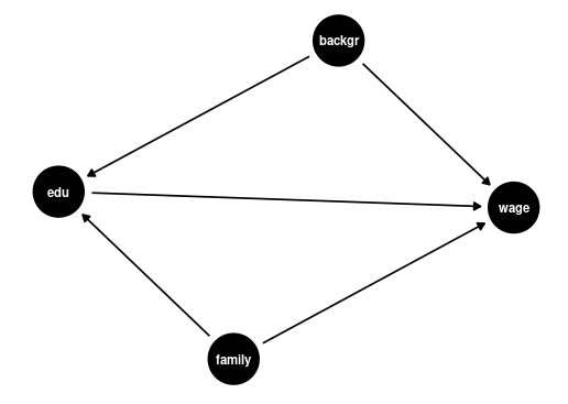
The coefficient \beta_2 is a measure of how strongly education and earnings are correlated.
This association could be due to other factors that correlate with both wages and education, such as family background (parental education, family income, ethnicity, structural racism) or personal background (gender, intelligence).
Notice: Correlation does not imply causation!
To disentangle the causal effect of education on wages from other correlative effects, we can include control variables.
9.2 Control Variables
To understand the causal effect of an additional year of education on wages, it is crucial to consider the influence of family and personal background. These factors, if not included in our analysis, are known as omitted variables. An omitted variable is one that:
- is correlated with the dependent variable (wage, in this scenario),
- is correlated with the regressor of interest (education),
- is omitted in the regression.
The presence of omitted variables means that we cannot be sure that the regression relationship between education and wages is purely causal. We say that we have omitted variable bias for the causal effect of the regressor of interest.
The coefficient \beta_2 in Equation 9.1 measures the correlative or marginal effect, not the causal effect. This must always be kept in mind when interpreting regression coefficients.
We can include control variables in the linear regression model to reduce omitted variable bias so that we can interpret \beta_2 as a ceteris paribus marginal effect (ceteris paribus means holding other variables constant).
For example, let’s include years of experience as well as racial background and gender dummy variables for Black and female: wage_i = \beta_1 + \beta_2 edu_i +\beta_3 exper_i + \beta_4 Black_i + \beta_5 fem_i + u_i. In this case, \beta_2 = \frac{\partial E[wage_i | edu_i, exper_i, Black_i, fem_i]}{\partial edu_i} is the marginal effect of education on expected wages, holding experience, race, and gender fixed.
lm(wage ~ education + experience + black + female, data = cps)
Call:
lm(formula = wage ~ education + experience + black + female,
    data = cps)

Coefficients:
(Intercept)    education   experience        black       female
   -21.7095       3.1350       0.2443      -2.8554      -7.4363
Interpretation: Given the same experience, racial background, and gender, people with one more year of education are paid on average 3.14 USD more than people with one year less of education.
Note: It does not hold other unobservable characteristics (such as ability) or variables not included in the regression (such as quality of education) fixed, so an omitted variable bias may still be present.
Good control variables are variables that are determined before the level of education is determined. Control variables should not be the cause of the dependent variable of interest.
Examples of good controls for education are parental education level, region of residence, or educational industry/field of study.
A problematic situation is when the control variable is the cause of education. Bad controls are typically highly correlated with the independent variable of interest and irrelevant to the causal effect of that variable on the dependent variable.
Examples of bad controls for education are current job position, number of professional certifications obtained, or number of job offers.
A high correlation of the bad control with the variable education also causes a high variance of the OLS coefficient for education and leads to an imprecise coefficient estimate. This problem is called imperfect multicollinearity.
Bad controls make it difficult to interpret causal relationships. They may control away the effect you want to measure, or they may introduce additional reverse causal effects hidden in the regression coefficients.
9.3 CASchools: class size effect
Recall the CASchools dataset used in the Stock and Watson textbook in sections 4-8.
data(CASchools, package = "AER")
CASchools$STR = CASchools$students/CASchools$teachers
CASchools$score = (CASchools$read+CASchools$math)/2
We are interested in the effect of the student-teacher ratio STR (class size) on the average test score score conditional on different control variables such as:
-
english: proportion of students whose primary language is not English. -
lunch: proportion of students eligible for free/reduced-price meals. -
expenditure: total expenditure per pupil.
                   STR      score     english       lunch expenditure
STR          1.0000000 -0.2263627  0.18764237  0.13520340 -0.61998216
score       -0.2263627  1.0000000 -0.64412381 -0.86877199  0.19127276
english      0.1876424 -0.6441238  1.00000000  0.65306072 -0.07139604
lunch        0.1352034 -0.8687720  0.65306072  1.00000000 -0.06103871
expenditure -0.6199822  0.1912728 -0.07139604 -0.06103871  1.00000000
The sample correlation matrix indicates that english, lunch and expenditure are correlated with STR and score, which implies these variables could confound the relationship of STR on score (omitted variable bias).
stargazer(fit1, fit2, fit3, fit4, type="html", report="vc*",
omit.stat = "f", star.cutoffs = NA)| Dependent variable: | ||||
| score | ||||
| (1) | (2) | (3) | (4) | |
| STR | -2.280 | -1.101 | -0.998 | -0.235 |
| english | -0.650 | -0.122 | -0.128 | |
| lunch | -0.547 | -0.546 | ||
| expenditure | 0.004 | |||
| Constant | 698.933 | 686.032 | 700.150 | 665.988 |
| Observations | 420 | 420 | 420 | 420 |
| R2 | 0.051 | 0.426 | 0.775 | 0.783 |
| Adjusted R2 | 0.049 | 0.424 | 0.773 | 0.781 |
| Residual Std. Error | 18.581 (df = 418) | 14.464 (df = 417) | 9.080 (df = 416) | 8.910 (df = 415) |
| Note: | NA | |||
Interpretations:
- Model (1): Between two classes that differ by one student, the class with more students scores on average 2.280 points lower.
- Model (2): Between two classes that differ by one student but have the same share of English learners, the larger class scores on average 1.101 points lower.
- Model (3): Between two classes that differ by one student but have the same share of English learners and students with reduced meals, the larger class scores on average 0.998 points lower.
- Model (4): Between two classes that differ by one student but have the same share of English learners, students with reduced meals, and per-pupil expenditure, the larger class scores on average 0.235 points lower.
The variables english and lunch are good controls because they are likely determined before class size decisions and capture important student background characteristics. These pre-existing factors can influence both class size assignments (as schools might create smaller classes for disadvantaged students) and test scores.
Per-pupil expenditure, however, is a bad control because it is likely determined simultaneously with or after class size decisions. Smaller classes mechanically increase per-pupil expenditure through higher teacher salary costs per student. Including expenditure therefore “controls away” part of the class size effect we aim to measure, which leads to potential underestimation of the true effect.
9.4 Polynomials
A linear dependence on wages and experience is a strong assumption. We can reasonably expect a nonlinear marginal effect of another year of experience on wages. For example, the effect may be higher for workers with 5 years of experience than for those with 40 years of experience.
Polynomials can be used to specify a nonlinear regression function: wage_i = \beta_1 + \beta_2 exper_i + \beta_3 exper_i^2 + \beta_4 exper_i^3 + u_i.
## we focus on people with Asian background only for illustration
cps.as = cps |> subset(asian == 1)
fit = lm(wage ~ experience + I(experience^2) + I(experience^3),
         data = cps.as)
beta = fit$coefficients
beta
(Intercept) experience I(experience^2) I(experience^3)
20.4547146896 1.2013241316 -0.0446897909 0.0003937551 ## Scatterplot
plot(wage ~ experience, data = cps.as, ylim = c(0,100))
## plot the cubic function for fitted wages
curve(
beta[1] + beta[2]*x + beta[3]*x^2 + beta[4]*x^3,
from = 0, to = 70, add=TRUE, col='red', lwd=2
)
The marginal effect depends on the years of experience: \frac{\partial E[wage_i | exper_i] }{\partial exper_i} = \beta_2 + 2 \beta_3 exper_i + 3 \beta_4 exper_i^2. For instance, the additional wage for a worker with 11 years of experience compared to a worker with 10 years of experience is on average 1.43 + 2\cdot (-0.042) \cdot 10 + 3 \cdot 0.0003 \cdot 10^2 = 0.68.
9.5 Interactions
A linear regression with interaction terms: wage_i = \beta_1 + \beta_2 edu_i + \beta_3 fem_i + \beta_4 marr_i + \beta_5 (marr_i \cdot fem_i) + u_i
lm(wage ~ education + female + married + married:female, data = cps)
Call:
lm(formula = wage ~ education + female + married + married:female,
    data = cps)

Coefficients:
   (Intercept)       education          female         married  female:married
       -17.886           2.867          -3.266           7.167          -5.767
The marginal effect of gender depends on the person’s marital status: \frac{\partial E[wage_i | edu_i, female_i, married_i] }{\partial female_i} = \beta_3 + \beta_5 married_i Interpretation: Given the same education, unmarried women are paid on average 3.27 USD less than unmarried men, and married women are paid on average 3.27+5.77=9.04 USD less than married men.
The marginal effect of the marital status depends on the person’s gender: \frac{\partial E[wage_i | edu_i, female_i, married_i]} {\partial married_i} = \beta_4 + \beta_5 female_i Interpretation: Given the same education, married men are paid on average 7.17 USD more than unmarried men, and married women are paid on average 7.17-5.77=1.40 USD more than unmarried women.
9.6 Logarithms
When analyzing wage data, we often use logarithmic transformations because they help model proportional relationships and reduce the skewness of the typically right-skewed distribution of wages. A common specification is the log-linear model, where we take the logarithm of wages while keeping education in its original scale:
In the logarithmic specification \log(wage_i) = \beta_1 + \beta_2 edu_i + u_i we have \frac{\partial E[\log(wage_i) | edu_i] }{\partial edu_i} = \beta_2.
This implies \underbrace{\partial E[\log(wage_i) | edu_i]}_{\substack{\text{absolute} \\ \text{change}}} = \beta_2 \cdot \underbrace{\partial edu_i}_{\substack{\text{absolute} \\ \text{change}}}. That is, \beta_2 gives the average absolute change in log-wages when education changes by 1.
Another interpretation can be given in terms of relative changes. Consider the following approximation: E[wage_i | edu_i] \approx \exp(E[\log(wage_i) | edu_i]). The left-hand expression is the conventional conditional mean, and the right-hand expression is the geometric mean. The geometric mean is slightly smaller because E[\log(Y)] < \log(E[Y]), but this difference is small unless the data is highly skewed.
The marginal effect of a change in edu on the geometric mean of wage is \frac{\partial exp(E[\log(wage_i) | edu_i])}{\partial edu_i} = \underbrace{exp(E[\log(wage_i) | edu_i])}_{\text{outer derivative}} \cdot \beta_2. Using the geometric mean approximation from above, we get \underbrace{\frac{\partial E[wage_i| edu_i] }{E[wage_i| edu_i]}}_{\substack{\text{percentage} \\ \text{change}}} \approx \frac{\partial exp(E[\log(wage_i) | edu_i])}{exp(E[\log(wage_i) | edu_i])} = \beta_2 \cdot \underbrace{\partial edu_i}_{\substack{\text{absolute} \\ \text{change}}}.
linear_model = lm(wage ~ education, data = cps.as)
log_model = lm(log(wage) ~ education, data = cps.as)
log_model
Call:
lm(formula = log(wage) ~ education, data = cps.as)

Coefficients:
(Intercept)    education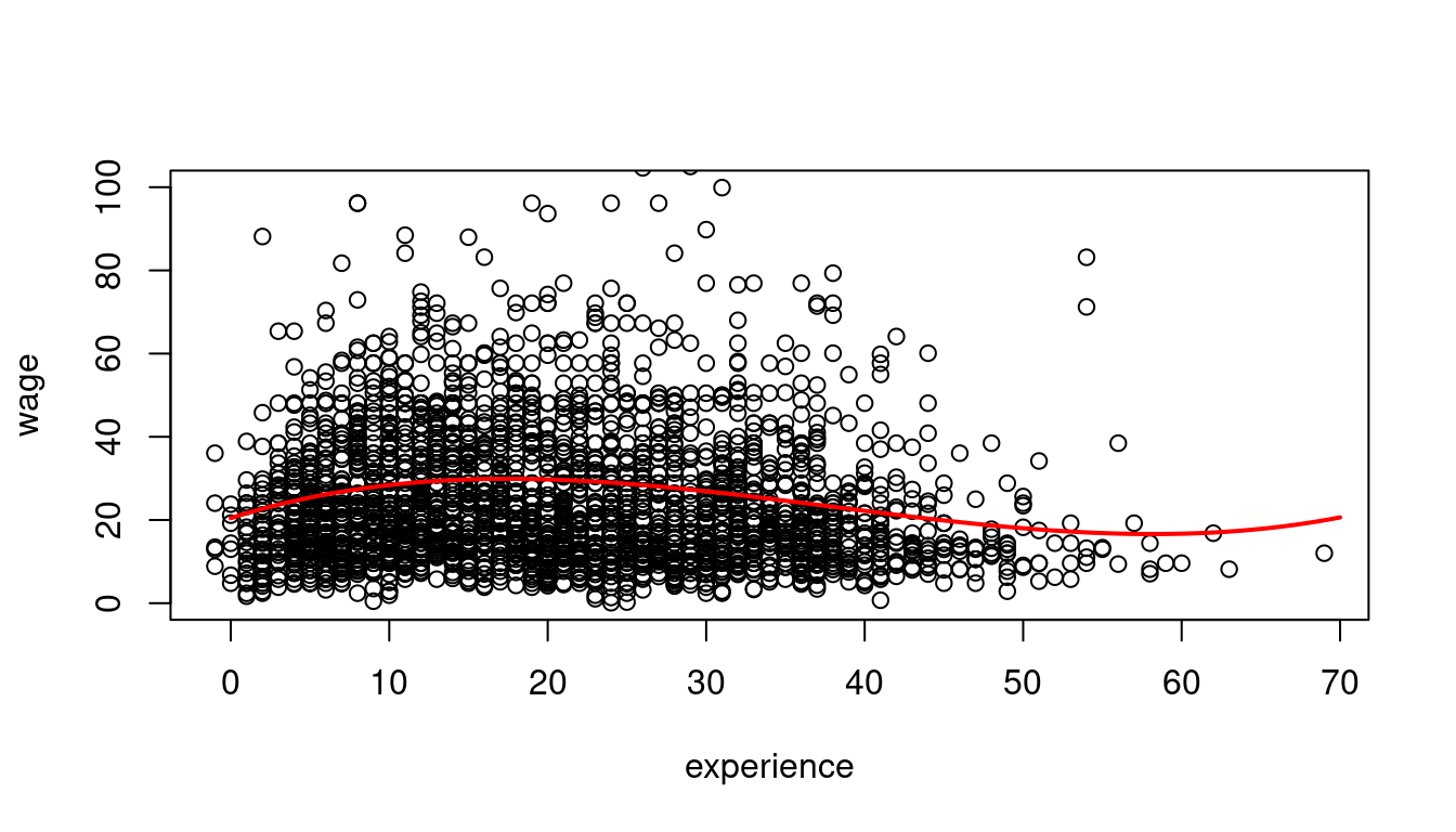
1.3783 0.1113 plot(wage ~ education, data = cps.as, ylim = c(0,80), xlim = c(4,22))
abline(linear_model, col="blue")
coef = coefficients(log_model)
curve(exp(coef[1]+coef[2]*x), add=TRUE, col="red")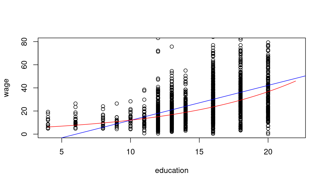
Interpretation: A person with one more year of education has a wage that is 11.13% higher on average.
In addition to the linear-linear and log-linear specifications, we also have the linear-log specification Y = \beta_1 + \beta_2 \log(X) + u and the log-log specification \log(Y) = \beta_1 + \beta_2 \log(X) + u.
Linear-log interpretation: When X is 1\% higher, we observe, on average, a 0.01 \beta_2 higher Y.
Log-log interpretation: When X is 1\% higher, we observe, on average, a \beta_2 \% higher Y.
9.7 CASchools: nonlinear specifications
Let’s have a look at an example that explores the relationship between the income of schooling districts and their test scores.
We start our analysis by computing the correlation between both variables.
cor(CASchools$income, CASchools$score)[1] 0.7124308Income and test score are positively correlated: school districts with above-average income tend to achieve above-average test scores. But does a linear regression adequately model the data? To investigate this further, let’s visualize the data by plotting them and adding a linear regression line.
# Create scatterplot
plot(score ~ income, data = CASchools,
    xlab = "District Income (thousands of USD)",
    ylab = "Test Score")
# Fit linear model and add regression line
linear = lm(score ~ income, data = CASchools)
abline(linear, col = "red", lwd = 2)
# Add legend
legend("bottomright", "Linear fit", col = "red", lwd = 2)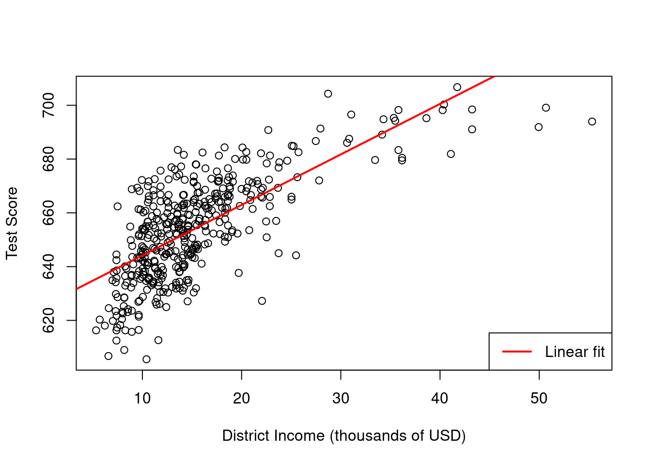
The plot shows that the linear regression line seems to overestimate the true relationship when income is either very high or very low and it tends to underestimates it for the middle income group. Luckily, OLS isn’t limited to linear regressions of the predictors. We have the flexibility to model test scores as a function of income and the square of income.
This leads us to the following regression model:
score_i = \beta_1 + \beta_2 \, income_i + \beta_3 \, income_i^2 + u_i which is a quadratic regression model. Here we treat income^2 as an additional explanatory variable.
Call:
lm(formula = score ~ income + I(income^2), data = CASchools)

Coefficients:
(Intercept)       income  I(income^2)
  607.30174      3.85099     -0.04231
The estimated function is
\widehat{score} = 607.3 \,+ 3.85 \, income - 0.0423 \, income^2
# Create scatterplot
plot(score ~ income, data = CASchools,
    xlab = "District Income (thousands)",
    ylab = "Test Score")

# Add fitted curves
curve(coef(linear)[1] + coef(linear)[2]*x, add = TRUE, col = "red", lwd=2)
curve(coef(quad)[1] + coef(quad)[2]*x + coef(quad)[3]*x^2, add = TRUE, col = "blue", lwd=2)

# Add legend
legend("bottomright", c("Quadratic", "Linear"), col = c("blue", "red"), lwd = 2)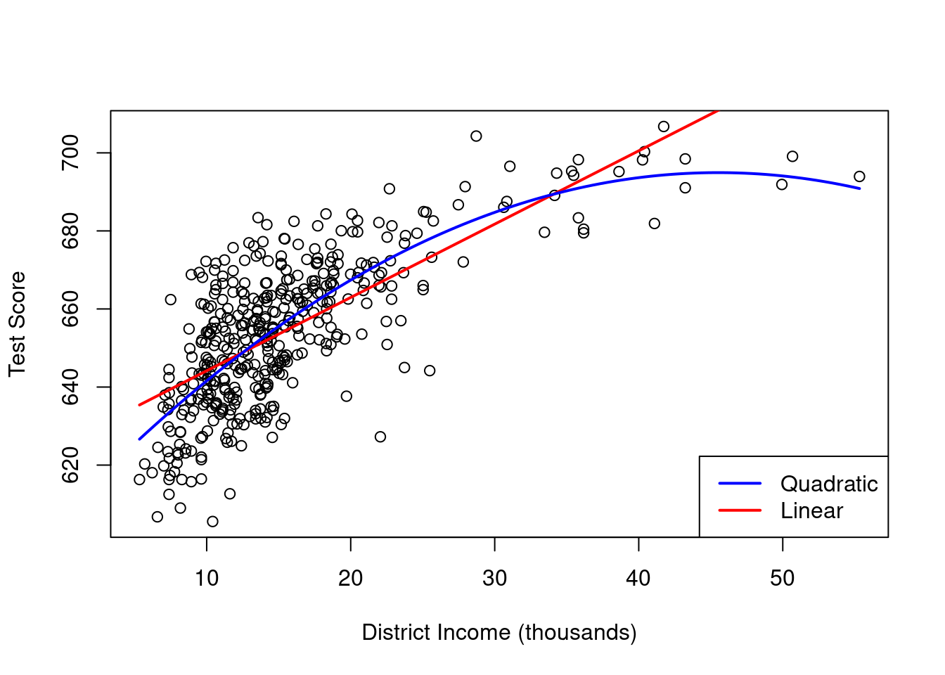
As the plot shows, the quadratic function appears to provide a better fit to the data compared to the linear function.
Another approach to estimate a concave nonlinear regression function involves using a logarithmic regressor.
Call:
lm(formula = score ~ log(income), data = CASchools)

Coefficients:
(Intercept)  log(income)
     557.83        36.42
The estimated regression model is
\widehat{score} = 557.8 + 36.42 \, \log (income)
# Create scatterplot
plot(score ~ income, data = CASchools,
    xlab = "Income", ylab = "Score")

# Add fitted curves
curve(coef(linlog)[1] + coef(linlog)[2]*log(x), add = TRUE, col = "blue", lwd = 2)
curve(coef(linear)[1] + coef(linear)[2]*x, add = TRUE, col = "red", lwd = 2)

# Add legend
legend("bottomright", c("Linear-log", "Linear"), col = c("blue", "red"), lwd = 2)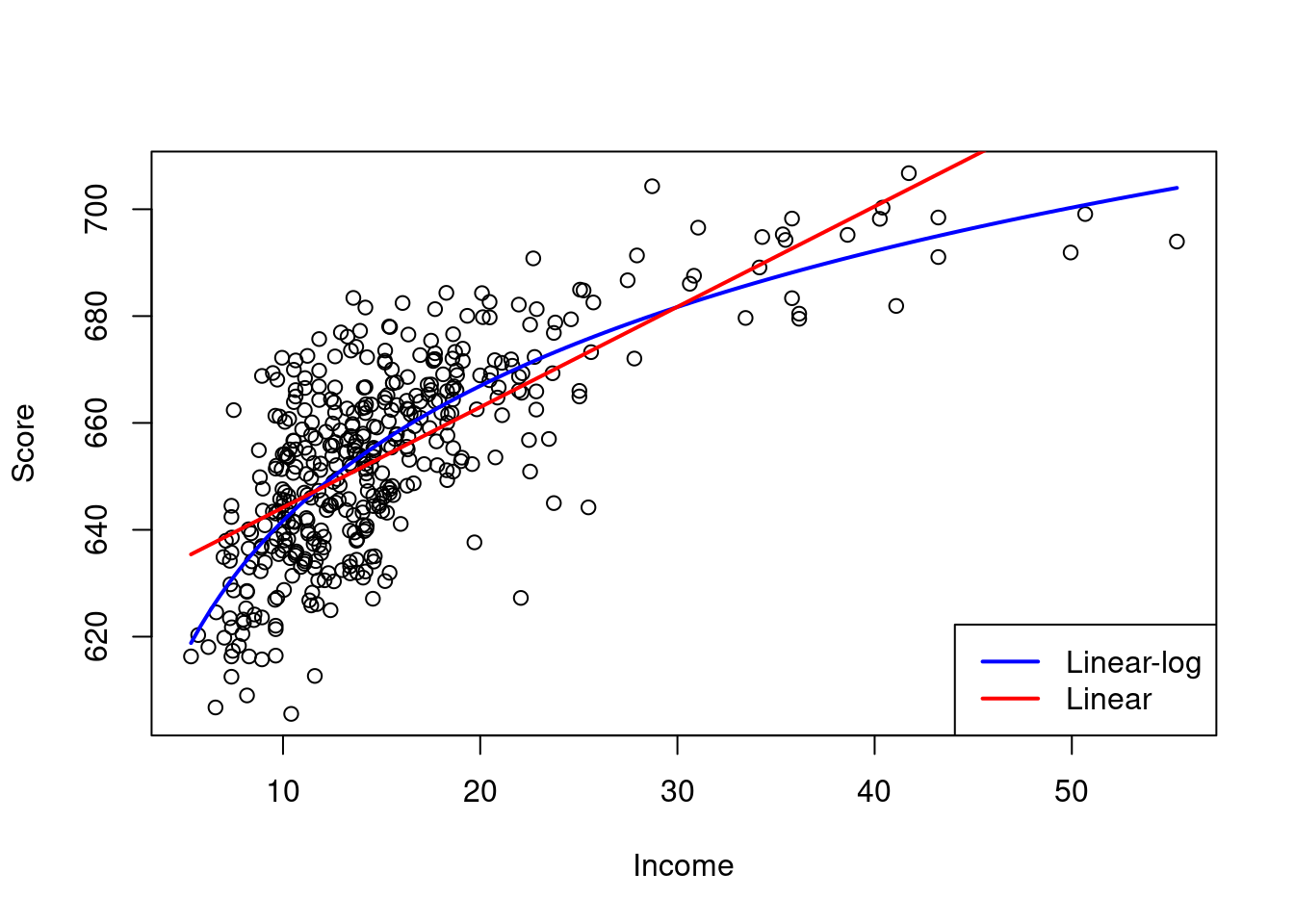
We can interpret \hat \beta_2 as follows: a 1\% increase in income is associated with an average increase in test scores of 0.01 \cdot 36.42 = 0.36 points.