7 Conditional expectation
7.1 Conditional distribution
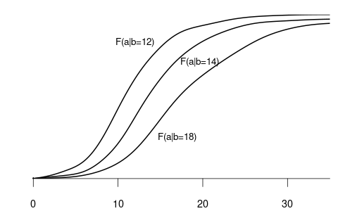
The conditional cumulative distribution function (conditional CDF), F_{Y|Z=b}(a) = F_{Y|Z}(a|b) = P(Y\leq a|Z=b), represents the distribution of a random variable Y given that another random variable Z takes a specific value b. It answers the question: “If we know that Z=b, what is the distribution of Y?”
For example, suppose that Y represents wage and Z represents education
- F_{Y|Z=12}(a) is the CDF of wages among individuals with 12 years of education.
- F_{Y|Z=14}(a) is the CDF of wages among individuals with 14 years of education.
- F_{Y|Z=18}(a) is the CDF of wages among individuals with 18 years of education.
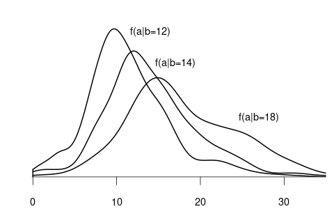
Since wage is a continuous variable, its conditional distribution given any specific value of another variable is also continuous. The conditional density of Y given Z=b is defined as the derivative of the conditional CDF: f_{Y|Z=b}(a) = f_{Y|Z}(a|b) = \frac{\partial}{\partial a} F_{Y|Z=b}(a).
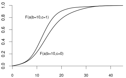
We can also condition on more than one variable. Let Z_1 represent the experience and Z_2 be the female dummy variable. The conditional CDF of Y given Z_1 = b and Z_2 = c is: F_{Y|Z_1=b,Z_2=c}(a).
For example:
- F_{Y|Z_1=10,Z_2=1}(a) is the CDF of wages among women with 10 years of experience.
- F_{Y|Z_1=10,Z_2=0}(a) is the CDF of wages among men with 10 years of experience.
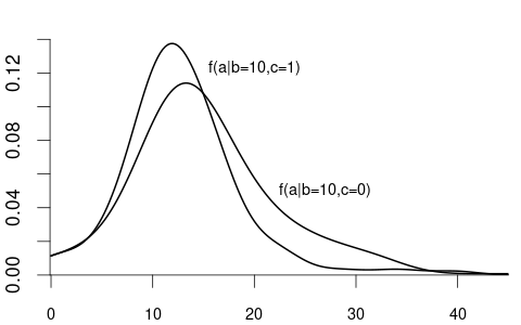
Similarly, we can take the derivative to get the conditional density f_{Y|Z_1=b, Z_2=c}(a):
More generally, we can condition on the event that a random vector \boldsymbol Z = (Z_1, \ldots, Z_k)' takes the value \{\boldsymbol Z = \boldsymbol b\}, i.e. \{Z_1 = b_1, \ldots, Z_k = b_k\}. The conditional CDF of Y given \{\boldsymbol Z = \boldsymbol b\} is F_{Y|\boldsymbol Z = \boldsymbol b}(a) = F_{Y|Z_1 = b_1, \ldots, Z_k = b_k}(a).
The variable of interest, Y, can also be discrete. Then, any conditional CDF of Y is also discrete. Below is the conditional CDF of education given the married dummy variable:
- F_{Y|Z=0}(a) is the CDF of education among unmarried individuals.
- F_{Y|Z=1}(a) is the CDF of education among married individuals.
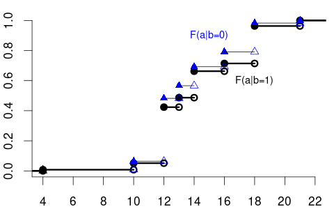
The conditional PMFs \pi_{Y|Z=0}(a) = P(Y = a | Z=0) and \pi_{Y|Z=1}(a)= P(Y = a | Z=1) indicate the jump heights of F_{Y|Z=0}(a) and F_{Y|Z=1}(a) at a.
7.1.1 Conditioning on discrete variables
If Z is a discrete random variable, then the conditional CDF can be expressed in terms of conditional probabilities.
The conditional probability of an event A given an event B with P(B) > 0 is P(A | B) = \frac{P(A \cap B)}{P(B)}
Let’s revisit the wage and schooling example from Table 4.3: \pi_{Y|Z=1}(1) = P(Y=1 | Z=1) = \frac{P(\{Y=1\}\cap \{Z=1\})}{P(Z=1)} = \frac{0.19}{0.36} = 0.53 \pi_{Y|Z=0}(1) = P(Y=1 | Z=0) = \frac{P(\{Y=1\}\cap \{Z=0\})}{P(Z=0)} = \frac{0.12}{0.64} = 0.19
Therefore, the conditional CDF of Y given \{Z=b\} with P(Z=b) > 0 is:
F_{Y|Z=b}(a) = P(Y \leq a| Z=b) = \frac{P(Y \leq a, Z=b)}{P(Z=b)} = \sum_{u \in \mathcal Y, u \leq a} \frac{\pi_{YZ}(u,b)}{\pi_{Z}(b)}.
7.1.2 Conditioning on continuous variables
If Z is a continuous variable, we have P(Z=b) = 0 for all b, and P(Y \leq a| Z=b) cannot be defined in the same way as for discrete variables.
If f_{YZ}(a,b) is the joint PDF of Y and Z and f_Z(b) is the marginal PDF of Z, the relation of the conditional CDF and the PDFs is as follows: F_{Y|Z=b}(a) = P(Y \leq a| Z=b) = \int_{-\infty}^a \frac{ f_{YZ}(u,b)}{f_Z(b)} \ \text{d}u.
7.2 Conditional mean
Conditional expectation
The conditional expectation or conditional mean of Y given \boldsymbol Z= \boldsymbol b is the expected value of the distribution F_{Y|\boldsymbol Z=\boldsymbol b}: E[Y | \boldsymbol Z= \boldsymbol b] = \int_{-\infty}^\infty a \ \text{d}F_{Y|\boldsymbol Z = \boldsymbol b}(a).
For continuous Y with conditional density f_{Y|\boldsymbol Z = \boldsymbol b}(a), we have \text{d}F_{Y|\boldsymbol Z = \boldsymbol b}(a) = f_{Y|\boldsymbol Z = \boldsymbol b}(a) \ \text{d}a, and the conditional expectation is E[Y | Z= \boldsymbol b] = \int_{-\infty}^\infty a f_{Y|\boldsymbol Z = \boldsymbol b}(a)\ \text{d}a. Similarly, for discrete Y with support \mathcal Y and conditional PMF \pi_{Y|\boldsymbol Z = \boldsymbol b}(a), we have E[Y | Z= \boldsymbol b] = \sum_{u \in \mathcal Y} u \pi_{Y|\boldsymbol Z = \boldsymbol b}(u).
The conditional expectation is a function of \boldsymbol b, which is a specific value of \boldsymbol Z that we condition on. Therefore, we call it the conditional expectation function: m(\boldsymbol b) = E[Y | Z= \boldsymbol b].
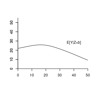
Suppose the conditional expectation of wage given experience level b is: m(b) = E[wage | exper = b] = 14.5 + 0.9 b - 0.017 b^2. For example, with 10 years of experience: m(10) = E[wage | exper = 10] = 21.8.
Here, m(b) assigns a specific real number to each fixed value of b; it is a deterministic function derived from the joint distribution of wage and experience.
However, if we treat experience as a random variable, the conditional expectation becomes: \begin{align*} m(exper) = E[wage | exper] = 14.5 + 0.9 exper - 0.017 exper^2. \end{align*} Now, m(exper) is a function of the random variable experexper and is itself a random variable.
In general:
- The conditional expectation given a specific value b is: m(\boldsymbol b) = E[Y | \boldsymbol Z=\boldsymbol b], which is deterministic.
- The conditional expectation given the random variable Z is:
m(\boldsymbol Z) = E[Y | \boldsymbol Z],
which is a random variable because it depends on the random vector \boldsymbol Z.
This distinction highlights that the conditional expectation can be either a specific number, i.e. E[Y | \boldsymbol Z=\boldsymbol b], or a random variable, i.e., E[Y | \boldsymbol Z], depending on whether the condition is fixed or random.
7.3 Rules of calculation
Let Y be a random variable and \boldsymbol{Z} a random vector. The rules of calculation rules below are fundamental tools for working with conditional expectations:
(i) Law of Iterated Expectations (LIE):
E[E[Y | \boldsymbol{Z}]] = E[Y].
Intuition: The LIE tells us that if we first compute the expected value of Y given each possible outcome of \boldsymbol{Z}, and then average those expected values over all possible values of \boldsymbol{Z}, we end up with the overall expected value of Y. It’s like calculating the average outcome across all scenarios by considering each scenario’s average separately.
More generally, for any two random vectors \boldsymbol{Z} and \boldsymbol{Z}^*:
E[E[Y | \boldsymbol{Z}, \boldsymbol{Z}^*] | \boldsymbol{Z}] = E[Y | \boldsymbol{Z}].
Intuition: Even if we condition on additional information \boldsymbol{Z}^*, averaging over \boldsymbol{Z}^* while keeping \boldsymbol{Z} fixed brings us back to the conditional expectation given \boldsymbol{Z} alone.
(ii) Conditioning Theorem (CT):
For any function g(\boldsymbol{Z}):
E[g(\boldsymbol{Z}) \, Y | \boldsymbol{Z}] = g(\boldsymbol{Z}) \, E[Y | \boldsymbol{Z}].
Intuition: Once we know \boldsymbol{Z}, the function g(\boldsymbol{Z}) becomes a known quantity. Therefore, when computing the conditional expectation given \boldsymbol{Z}, we can treat g(\boldsymbol{Z}) as a constant and factor it out.
(iii) Independence Rule (IR):
If Y and \boldsymbol{Z} are independent, then:
E[Y | \boldsymbol{Z}] = E[Y].
Intuition: Independence means that Y and \boldsymbol{Z} do not influence each other. Knowing the value of \boldsymbol{Z} gives us no additional information about Y. Therefore, the expected value of Y remains the same regardless of the value of \boldsymbol{Z}, so the conditional expectation equals the unconditional expectation.
Another way to see this is the fact that, if Y and Z are independent, then F_{Y|Z=b}(a) = F_{Y}(a) \quad \text{for all} \ a \ \text{and} \ b.
7.4 Best predictor property
It turns out that the CEF m(\boldsymbol Z) = E[Y | \boldsymbol Z] is the best predictor for Y given the information contained in the random vector \boldsymbol Z:
Best predictor
The CEF m(\boldsymbol Z) = E[Y | \boldsymbol Z] minimizes the expected squared error E[(Y-g(\boldsymbol Z))^2] among all predictor functions g(\boldsymbol Z): m(\boldsymbol Z) = \argmin_{g(\boldsymbol Z)} E[(Y-g(\boldsymbol Z))^2]
Proof: Let us find the function g(\cdot) that minimizes E[(Y-g(\boldsymbol Z))^2]:
\begin{align*} &E[(Y-g(\boldsymbol Z))^2] = E[(Y-m(\boldsymbol Z) + m(\boldsymbol Z) - g(\boldsymbol Z))^2] \\ &= \underbrace{E[(Y-m(\boldsymbol Z))^2]}_{=(i)} + 2\underbrace{E[(Y-m(\boldsymbol Z))(m(\boldsymbol Z) - g(\boldsymbol Z))]}_{=(ii)} + \underbrace{E[(m(\boldsymbol Z) - g(\boldsymbol Z))^2]}_{(iii)} \end{align*}
- The first term (i) does not depend on g(\cdot) and is finite if E[Y^2] < \infty.
- For the second term (ii), we use the LIE and CT: \begin{align*} &E[(Y-m(\boldsymbol Z))(m(\boldsymbol Z) - g(\boldsymbol Z))] \\ &= E[E[(Y-m(\boldsymbol Z))(m(\boldsymbol Z) - g(\boldsymbol Z))| \boldsymbol Z]] \\ &= E[E[Y-m(\boldsymbol Z)| \boldsymbol Z](m(\boldsymbol Z) - g(\boldsymbol Z))] \\ &= E[(\underbrace{E[Y| \boldsymbol Z]}_{=m(\boldsymbol Z)} - m(\boldsymbol Z))(m(\boldsymbol Z) - g(\boldsymbol Z))] = 0 \end{align*}
- The third term (iii) E[(m(\boldsymbol Z) - g(\boldsymbol Z))^2] is minimal if g(\cdot) = m(\cdot).
Therefore, m(\boldsymbol Z) = E[Y| \boldsymbol Z] minimizes E[(Y-g(\boldsymbol Z))^2].
The best predictor for Y given \boldsymbol Z is m(\boldsymbol Z)= E[Y | \boldsymbol Z], but Y can typically only partially be predicted. We have a prediction error (CEF error) u = Y - E[Y | \boldsymbol Z]. The conditional expectation of the CEF error does not depend on X and is zero: \begin{align*} E[u | \boldsymbol Z] &= E[(Y - m(\boldsymbol Z)) | \boldsymbol Z] \\ &= E[Y | \boldsymbol Z] - E[m(\boldsymbol Z) | \boldsymbol Z] \\ &= m(\boldsymbol Z) - m(\boldsymbol Z) = 0. \end{align*}
7.5 Linear regression model
Consider again the linear regression framework with dependent variable Y_i and regressor vector \boldsymbol X_i. The previous section shows that we can always write Y_i = m(\boldsymbol X_i) + u_i, \quad E[u_i | \boldsymbol X_i] = 0, where m(\boldsymbol X_i) is the CEF of Y_i given \boldsymbol X_i, and u_i is the CEF error.
In the linear regression model, we assume that the CEF is linear in \boldsymbol X_i, i.e. Y_i = \boldsymbol X_i'\boldsymbol \beta + u_i, \quad E[u_i | \boldsymbol X_i] = 0. From this equation, by the CT, it becomes clear that E[Y_i | \boldsymbol X_i] = E[\boldsymbol X_i'\boldsymbol \beta + u_i| \boldsymbol X_i] = \boldsymbol X_i'\boldsymbol \beta + E[u_i | \boldsymbol X_i] = \boldsymbol X_i'\boldsymbol \beta. Therefore, \boldsymbol X_i'\boldsymbol \beta is the best predictor for Y_i given \boldsymbol X_i.
Linear regression model
We assume that (Y_i, \boldsymbol X_i') satisfies Y_i = \boldsymbol X_i'\boldsymbol \beta + u_i, \quad i=1, \ldots, n, \tag{7.1} with
(A1) conditional mean independence: E[u_i | \boldsymbol X_i] = 0
(A2) random sampling: (Y_i, \boldsymbol X_i') are i.i.d. draws from their joint population distribution
(A3) large outliers unlikely: 0 < E[Y_i^4] < \infty, 0 < E[X_{il}^4] < \infty for all l=1, \ldots, k
(A4) no perfect multicollinearity: \sum_{i=1}^n \boldsymbol X_i \boldsymbol X_i' is invertible
In matrix notation, the model equation can be written as \boldsymbol Y = \boldsymbol X \boldsymbol \beta + \boldsymbol u, where \boldsymbol u = (u_1, \ldots, u_n)' is the error term vector, \boldsymbol Y is the dependent variable vector, and \boldsymbol X is the n \times k regressor matrix.
(A1) and (A2) define the structure of the regression model, while (A3) and (A4) ensure that OLS estimation is feasible and reliable.
7.5.1 Conditional mean independence (A1)
Assumption (A1) is fundamental to the regression model and has several key implications:
1) Zero unconditional mean
Using the Law of Iterated Expectations (LIE): E[u_i] \overset{\tiny (LIE)}{=} E[E[u_i | \boldsymbol X_i]] = E[0] = 0
The error term u_i has a zero unconditional mean.
2) Linear best predictor
The conditional mean of Y_i given X_{i} is: \begin{align*} E[Y_i | \boldsymbol X_i] &= E[\boldsymbol X_i'\boldsymbol \beta + u_i | \boldsymbol X_i] \\ &\overset{\tiny (CT)}{=} \boldsymbol X_i'\boldsymbol \beta + E[u_i | \boldsymbol X_i] \\ &= \boldsymbol X_i'\boldsymbol \beta \end{align*}
The regression function \boldsymbol X_i'\boldsymbol \beta represents the best linear predictor of Y_i given \boldsymbol X_i. This means the expected value of Y_i is a linear function of the regressors.
3) Marginal effect interpretation
From the linearity of the conditional expectation: E[Y_i | \boldsymbol X_i] = \boldsymbol X_i'\boldsymbol \beta = \beta_1 + \beta_2 X_{i2} + \ldots + \beta_k X_{ik}. The partial derivative with respect to X_{ij} is: \frac{\text{d} E[Y_i | \boldsymbol X_i]}{ \text{d} X_{ij}} = \beta_j
The coefficient \beta_j represents the marginal effect of a one-unit increase in X_{ij} on the expected value of Y_i, holding all other variables constant.
Note: This marginal effect is not necessarily causal. Unobserved factors correlated with X_{ij} may influence Y_i, so \beta_j captures both the direct effect of X_{ij} and the indirect effect through these unobserved variables.
4) Weak exogeneity
Using the definition of covariance: Cov(u_i, X_{il}) = E[u_i X_{il}] - E[u_i] E[X_{il}]. Since E[u_i] = 0: Cov(u_i, X_{il}) = E[u_i X_{il}]. Applying the LIE and the CT: \begin{align*} E[u_i X_{il}] &= E[E[u_i X_{il}|\boldsymbol X_i]] \\ &= E[X_{il} E[u_i|\boldsymbol X_i]] \\ &= E[X_{il} \cdot 0] = 0 \end{align*}
The error term u_i is uncorrelated with each regressor X_{il}. This property is known as weak exogeneity. It indicates that u_ii captures unobserved factors that do not systematically vary with the observed regressors.
Note: Weak exogeneity does not rule out the presence of unobserved variables that affect both Y_i and \boldsymbol X_i. The coefficient \beta_j reflects the average relationship between \boldsymbol X_i and Y_i, including any indirect effects from unobserved factors that are correlated with \boldsymbol X_i.
7.5.2 Random sampling (A2)
1) Strict exogeneity
The i.i.d. assumption (A2) implies that \{(Y_i, \boldsymbol X_i',u_i), i=1,\ldots,n\} is an i.i.d. collection since u_i = Y_i - \boldsymbol X_i'\boldsymbol \beta is a function of a random sample, and functions of independent variables are independent as well.
Therefore, u_i and \boldsymbol X_j are independent for i \neq j. The independence rule (IR) implies E[u_i | \boldsymbol X_1, \ldots, \boldsymbol X_n] = E[u_i | \boldsymbol X_i].
The weak exogeneity condition (A1) turns into a strict exogeneity property: E[u_i | \boldsymbol X] = E[u_i | \boldsymbol X_1, \ldots, \boldsymbol X_n] \overset{\tiny (A2)}{=} E[u_i | \boldsymbol X_i] \overset{\tiny (A1)}{=} 0. Additionally, Cov(u_j, X_{il}) = \underbrace{E[u_j X_{il}]}_{=0} - \underbrace{E[u_j]}_{=0} E[X_{il}] = 0.
Weak exogeneity means that the regressors of individual i are uncorrelated with the error term of the same individual i. Strict exogeneity means that the regressors of individual i are uncorrelated with the error terms of any individual j in the sample.
2) Heteroskedasticity
The i.i.d. assumption (A2) is not as restrictive as it may seem at first sight. It allows for dependence between u_i and \boldsymbol X_i = (1,X_{i2},\dots,X_{ik})'. The error term u_i can have a conditional distribution that depends on \boldsymbol X_i.
The exogeneity assumption (A1) requires that the conditional mean of u_i is independent of \boldsymbol X_i. Besides this, dependencies between u_i and X_{i2},\dots,X_{ik} are allowed. For instance, the variance of u_i can be a function of X_{i2},\dots,X_{ik}. If this is the case, u_i is said to be heteroskedastic.
The conditional variance is defined analogously to the unconditional variance: Var[Y|\boldsymbol Z] = E[(Y-E[\boldsymbol Y|\boldsymbol Z])^2|\boldsymbol Z] = E[Y^2|\boldsymbol Z] - E[Y|\boldsymbol Z]^2.
The conditional variance of the error is: Var[u_i | \boldsymbol X] = E[u_i^2 | \boldsymbol X] \overset{\tiny (A2)}{=} E[u_i^2 | \boldsymbol X_i] =: \sigma_i^2 = \sigma^2(\boldsymbol X_i). An additional restrictive assumption is homoskedasticity, which means that the variance of u_i is not allowed to vary for different values of \boldsymbol X_i: Var[u_i | \boldsymbol X] = \sigma^2. Homoskedastic errors are a restrictive assumption sometimes made for convenience in addition to (A1)+(A2). Homoskedasticity is often unrealistic in practice, so we stick with the heteroskedastic errors framework.
3) No autocorrelation
(A2) implies that u_i is independent of u_j for i \neq j, and therefore E[u_i | u_j, \boldsymbol X] = E[u_i | \boldsymbol X] = 0 by the IR. This implies
E[u_i u_j | \boldsymbol X] \overset{\tiny (LIE)}{=} E\big[E[u_i u_j | u_j, \boldsymbol X] | \boldsymbol X\big] \overset{\tiny (CT)}{=} E\big[u_j \underbrace{E[u_i | u_j, \boldsymbol X]}_{=0} | \boldsymbol X\big] = 0, and, therefore, Cov(u_i, u_j) = E[u_i u_j] \overset{\tiny (LIE)}{=} E[E[u_i u_j | \boldsymbol X]] = 0.
The conditional covariance matrix of the error term vector \boldsymbol u is \boldsymbol D := Var[\boldsymbol u | \boldsymbol X] = E[\boldsymbol u \boldsymbol u' | \boldsymbol X] = \begin{pmatrix} \sigma_1^2 & 0 & \ldots & 0 \\ 0 & \sigma_2^2 & \ldots & 0 \\ \vdots & \vdots & \ddots & \vdots \\ 0 & 0 & \ldots & \sigma_n^2 \end{pmatrix}.
It is a diagonal matrix with conditional variances on the main diagonal. We also write \boldsymbol D = diag(\sigma_1^2, \ldots, \sigma_n^2).
7.5.3 Finite moments and invertibility (A3 + A4)
Assuming (A3) excludes frequently occurring large outliers as it rules out heavy-tailed distributions. Hence, we should be careful if we use variables with large kurtosis. Assuming (A4) ensures that the OLS estimator \widehat{\boldsymbol \beta} can be computed.
7.5.3.1 Unbiasedness
(A4) ensures that \widehat{\boldsymbol \beta} is well defined. The following decomposition is useful: \begin{align*} \widehat{\boldsymbol \beta} &= (\boldsymbol X' \boldsymbol X)^{-1} \boldsymbol X' \boldsymbol Y \\ &= (\boldsymbol X' \boldsymbol X)^{-1} \boldsymbol X' (\boldsymbol X \boldsymbol \beta + \boldsymbol u) \\ &= (\boldsymbol X' \boldsymbol X)^{-1} (\boldsymbol X' \boldsymbol X) \boldsymbol \beta + (\boldsymbol X' \boldsymbol X)^{-1} \boldsymbol X' \boldsymbol u \\ &= \boldsymbol \beta + (\boldsymbol X' \boldsymbol X)^{-1} \boldsymbol X' \boldsymbol u. \end{align*} The strict exogeneity implies E[\boldsymbol u | \boldsymbol X] = \boldsymbol 0, and E[\widehat{ \boldsymbol \beta} - \boldsymbol \beta | \boldsymbol X] = E[(\boldsymbol X' \boldsymbol X)^{-1} \boldsymbol X' \boldsymbol u | \boldsymbol X] \overset{\tiny (CT)}{=} (\boldsymbol X' \boldsymbol X)^{-1} \boldsymbol X' \underbrace{E[\boldsymbol u | \boldsymbol X]}_{= \boldsymbol 0} = \boldsymbol 0. By the (LIE), E[\widehat{ \boldsymbol \beta}] = E[E[\widehat{ \boldsymbol \beta} | \boldsymbol X]] = E[\boldsymbol \beta] = \boldsymbol \beta.
Hence, the OLS estimator is unbiased: Bias[\widehat{\boldsymbol \beta}] = 0.
7.5.3.2 Conditional variance
Recall the matrix rule Var[\boldsymbol A \boldsymbol Z] = \boldsymbol A Var[\boldsymbol Z] \boldsymbol A' if \boldsymbol Z is a random vector and \boldsymbol A is a matrix. Then, \begin{align*} Var[\widehat{ \boldsymbol \beta} | \boldsymbol X] &= Var[\boldsymbol \beta + (\boldsymbol X'\boldsymbol X)^{-1} \boldsymbol X' \boldsymbol u | \boldsymbol X] \\ &= Var[(\boldsymbol X'\boldsymbol X)^{-1} \boldsymbol X' \boldsymbol u | \boldsymbol X] \\ &= (\boldsymbol X'\boldsymbol X)^{-1} \boldsymbol X' Var[\boldsymbol u | \boldsymbol X] ((\boldsymbol X'\boldsymbol X)^{-1} \boldsymbol X')' \\ &= (\boldsymbol X'\boldsymbol X)^{-1} \boldsymbol X' \boldsymbol D \boldsymbol X (\boldsymbol X'\boldsymbol X)^{-1}. \end{align*}
7.5.3.3 Consistency
The conditional variance can be written as \begin{align*} Var[\widehat{ \boldsymbol \beta} | \boldsymbol X] &= \frac{1}{n} \Big( \frac{1}{n} \boldsymbol X' \boldsymbol X \Big)^{-1} \Big(\frac{1}{n} \boldsymbol X' \boldsymbol D \boldsymbol X \Big) \Big( \frac{1}{n} \boldsymbol X' \boldsymbol X \Big)^{-1} \\ &= \frac{1}{n} \Big( \frac{1}{n} \sum_{i=1}^n \boldsymbol X_i \boldsymbol X_i' \Big)^{-1} \Big(\frac{1}{n} \sum_{i=1}^n \sigma_i^2 \boldsymbol X_i \boldsymbol X_i' \Big) \Big( \frac{1}{n} \sum_{i=1}^n \boldsymbol X_i \boldsymbol X_i' \Big)^{-1} \end{align*}
It can be shown, by the multivariate law of large numbers, that \frac{1}{n} \sum_{i=1}^n \boldsymbol X_i \boldsymbol X_i' \overset{p}{\rightarrow} E[\boldsymbol X_i \boldsymbol X_i'] and \sum_{i=1}^n \sigma_i^2 \boldsymbol X_i \boldsymbol X_i \overset{p}{\rightarrow} E[\sigma_i^2 \boldsymbol X_i \boldsymbol X_i']. For this to hold we need bounded fourth moments, i.e. (A3). In total, we have \begin{align*} &\Big( \frac{1}{n} \sum_{i=1}^n \boldsymbol X_i \boldsymbol X_i' \Big)^{-1} \Big(\frac{1}{n} \sum_{i=1}^n \sigma_i^2 \boldsymbol X_i \boldsymbol X_i' \Big) \Big( \frac{1}{n} \sum_{i=1}^n \boldsymbol X_i \boldsymbol X_i' \Big)^{-1} \\ &\overset{p}{\rightarrow} E[\boldsymbol X_i \boldsymbol X_i']^{-1} E[\sigma_i^2 \boldsymbol X_i \boldsymbol X_i'] E[\boldsymbol X_i \boldsymbol X_i']^{-1}. \end{align*} Note that the conditional variance Var[\widehat{ \boldsymbol \beta} | \boldsymbol X] has an additional factor 1/n, which converges to zero for large n. Therefore, we have Var[\widehat{ \boldsymbol \beta} | \boldsymbol X] \overset{p}{\rightarrow} \boldsymbol 0, which also holds for the unconditional variance, i.e. Var[\widehat{ \boldsymbol \beta}] \to \boldsymbol 0.
Therefore, since the bias is zero and the variance converges to zero, the sufficient conditions for consistency are fulfilled. The OLS estimator \widehat{\boldsymbol \beta} is a consistent estimator for \boldsymbol \beta under (A1)–(A4).