| ISCED level | Education level | Years of schooling |
|---|---|---|
| 1 | Primary | 4 |
| 2 | Lower Secondary | 10 |
| 3 | Upper secondary | 12 |
| 4 | Post-Secondary | 13 |
| 5 | Short-Cycle Tertiary | 14 |
| 6 | Bachelor's | 16 |
| 7 | Master's | 18 |
| 8 | Doctoral | 21 |
4 Probability
4.1 Random sampling
From the perspective of empirical analysis, a dataset Y_1, \ldots, Y_n or \boldsymbol X_1, \ldots, \boldsymbol X_n is simply an array of fixed numbers presented to a researcher. The summary statistics we compute – such as sample means, sample correlations, and OLS coefficients – are functions of this given dataset.
While these statistics provide a snapshot of the data at hand, they do not automatically offer insights into the broader world from which the data originated. To add deeper meaning to these numbers and draw conclusions about underlying dependencies and causalities, we need to consider how the data were obtained.
In statistical theory, a dataset is viewed as the result of a random experiment. The gender of the next person you meet, daily fluctuations in stock prices, monthly music streams of your favorite artist, or the annual number of pizzas consumed – all involve a certain amount of randomness.
Sampling refers to the process of obtaining data by drawing observations from a population, which is often considered infinite in statistical theory. An infinite population is a theoretical construct, representing not just the existing physical population but all possible future or hypothetical individuals.

This figure demonstrates the concept of sampling. The left side displays the full set of letters from “a” to “z”, representing the entire (infinite) population. From this population, five letters are randomly chosen, forming the sample shown on the right side.
The goal of statistical inference is to learn about the underlying population distribution by analyzing the observed sample. To do so, we need to make assumptions about how the data were sampled.
The simplest and ideal case is random sampling, where observations are randomly drawn from this infinite distribution with replacement – like randomly drawing balls from an urn, or randomly selecting individuals for a representative survey. This principle is also known as i.i.d. sampling (independent and identically distributed sampling). To define these concepts rigorously, we require probability theory.
4.2 Random variables
A random variable is a numerical summary of a random experiment. An outcome is a specific result of a random experiment. The sample space S is the set/collection of all potential outcomes.
Let’s consider some examples:
- Coin toss: The outcome of a coin toss can be “heads” or “tails”. This random experiment has a two-element sample space: S = \{heads, tails\}. We can express the experiment as a binary random variable: Y = \begin{cases} 1 & \text{if outcome is heads,} \\ 0 & \text{if outcome is tails.} \end{cases}
- Gender: If you conduct a survey and interview a random person to ask them about their gender, the answer may be “female”, “male”, or “diverse”. It is a random experiment since the person to be interviewed is selected randomly. The sample space has three elements: S = \{female, male, diverse\}. To focus on female vs. non-female, we can define the female dummy variable: Y = \begin{cases} 1 & \text{if the person is female,} \\ 0 & \text{if the person is not female.} \end{cases} Similarly, dummy variables for male and diverse can be defined.
- Education level: If you ask a random person about their education level according to the ISCED-2011 framework, the outcome may be one of the eight ISCED-2011 levels. We have an eight-element sample space: S = \{Level \ 1, Level \ 2, Level \ 3, Level \ 4, Level \ 5, Level \ 6, Level \ 7, Level \ 8\}. The eight-element sample space of the education-level random experiment provides a natural ordering. We define the random variable education as the number of years of schooling of the interviewed person: Y = \text{number of years of schooling} \in \{4, 10, 12, 13, 14, 16, 18, 21\}.
- Wage: If you ask a random person about their income per working hour in EUR, there are infinitely many potential answers. Any (non-negative) real number may be an outcome. The sample space is a continuum of different wage levels. The wage level of the interviewed is already numerical. The random variable is Y = \text{income per working hour in EUR}.
These random variables have in common that they take values on the real line \mathbb R but their outcome is uncertain before conducting the random experiment (i.e. flipping the coin or selecting a random person to be interviewed).
4.3 Events and probabilities
An event of a random variable Y is a specific subset of the real line. Any real number defines an event (elementary event), and any open, half-open, or closed interval represents an event as well.
Let’s define some specific events:
- Elementary events: A_1 = \{Y=0\}, \quad A_2 = \{Y=1\}, \quad A_3 = \{Y=2.5\}
- Half-open events: \begin{align*} A_4 &= \{Y \geq 0\} = \{ Y \in [0,\infty) \} \\ A_5 &= \{ -1 \leq Y < 1 \} = \{ Y \in [-1,1) \}. \end{align*}
The probability function P assigns values between 0 and 1 to events. It is natural to assign the following probabilities for a fair coin toss: P(A_1) = P(Y=0) = 0.5, \quad P(A_2) = P(Y=1) = 0.5 By definition, the coin variable will never take the value 2.5, so we assign P(A_3) = P(Y=2.5) = 0. For each intervals, we check whether the events \{Y=0\} and/or \{Y=1\} are subsets of the event of interest. If both \{Y=0\} and \{Y=1\} are contained in the event, the probability is 1. If only one of them is contained, the probability is 0.5. If neither is contained, the probability is 0. P(A_4) = P(Y \geq 0) = 1, \quad P(A_5) = P( -1 \leq Y < 1) = 0.5.
Every event has a complementary event, and for any pair of events we can take the union and intersection. Let’s define further events:
- Complements: A_6 = A_4^c = \{Y \geq 0\}^c = \{ Y < 0\} = \{Y \in (-\infty, 0)\},
- Unions: A_7 = A_1 \cup A_6 = \{Y=0\} \cup \{Y< 0\} = \{Y \leq 0\}
- Intersections: A_8 = A_4 \cap A_5 = \{Y \geq 0\} \cap \{ -1 \leq Y < 1 \} = \{ 0 \leq Y < 1 \}
- Iterations of it: A_9 = A_1 \cup A_2 \cup A_3 \cup A_5 \cup A_6 \cup A_7 \cup A_8 = \{ Y \in (-\infty, 1] \cup \{2.5\}\},
- Certain event: A_{10} = A_9 \cup A_9^c = \{Y \in (-\infty, \infty)\} = \{Y \in \mathbb R\}
- Empty event: A_{11} = A_{10}^c = \{ Y \notin \mathbb R \} = \{ \}
You may verify that P(A_1) = 0.5, P(A_2) = 0.5, P(A_3) = 0, P(A_4) = 1 P(A_5) = 0.5, P(A_6) = 0, P(A_7) = 0.5, P(A_8) = 0.5, P(A_9) = 1, P(A_{10}) = 1, P(A_{11}) = 0 for the coin toss experiment. If you take the variables education or wage, the probabilities of these events will be completely different.
4.4 Probability function
The Borel sigma algebra \mathcal B is the collection of all events to which we assign probabilities. The events A_1, \ldots, A_{11} mentioned earlier are elements of \mathcal B. Any event of the form \{ Y \in (a,b) \}, where a, b \in \mathbb{R}, is also an element of \mathcal B. Furthermore, all possible unions, intersections, and complements of these events are contained in \mathcal B. In essence, \mathcal B can be thought of as the comprehensive collection of all events for which we would ever compute probabilities in practice.
The following mathematical axioms ensure that the concept of probability is well-defined and possesses the desired properties:
Probability function
A probability function P is a function P: \mathcal B \to [0,1] that satisfies the Axioms of Probability:
P(A) \geq 0 for every A \in \mathcal B
P(Y \in \mathbb R) = 1
If A_1, A_2, A_3 \ldots are disjoint then A_1 \cup A_2 \cup A_3 \cup \ldots = P(A_1) + P(A_2) + P(A_3) + \ldots
Two events A and B are disjoint if A \cap B = \{\}, i.e., if they have no outcomes in common. For instance, A_1 = \{Y=0\} and A_2 = \{Y=1\} are disjoint, but A_1 and A_4 = \{Y \geq 0\} are not disjoint, since A_1 \cap A_4 = \{Y=0\} is nonempty.
The axioms of probability imply the following rules of calculation:
Basic rules of probability
- 0 \leq P(A) \leq 1 for any event A
- P(A) \leq P(B) if A is a subset of B
- P(A^c) = 1 - P(A) for the complement event of A
- P(A \cup B) = P(A) + P(B) - P(A \cap B) for any events A, B
- P(A \cup B) = P(A) + P(B) if A and B are disjoint
4.5 Distribution function
Assigning probabilities to events is straightforward for binary variables, like coin tosses. For instance, knowing that P(Y = 1) = 0.5 allows us to derive the probabilities for all events in \mathcal B. However, for more complex variables, such as education or wage, defining probabilities for all possible events becomes more challenging due to the vast number of potential set operations involved.
Fortunately, it turns out that knowing the probabilities of events of the form \{Y \leq a\} is enough to determine the probabilities of all other events. These probabilities are summarized in the cumulative distribution function.
Cumulative distribution function (CDF)
The cumulative distribution function (CDF) of a random variable Y is F(a) := P(Y \leq a), \quad a \in \mathbb R.
The CDF is sometimes referred to as the distribution function, or simply the distribution. The distribution defines the probabilities for all possible events in \mathcal B.
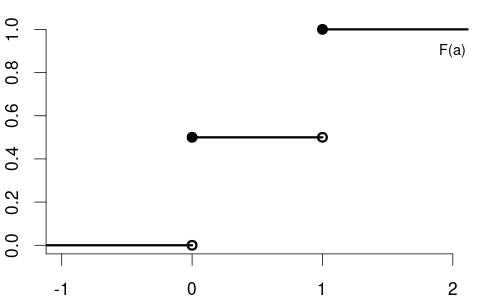
The CDF of the variable coin is F(a) = \begin{cases} 0 & a < 0, \\ 0.5 & 0 \leq a < 1, \\ 1 & a \geq 1, \end{cases} with the following CDF plot:
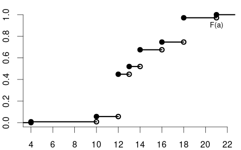
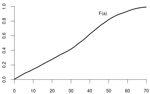
The CDF of the variable education may be
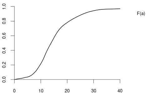
and the CDF of the variable wage may have the following form:
By the basic rules of probability, we can compute the probability of any event of interest if we know the probabilities of all events of the forms \{Y \leq a\} and \{Y = a \}.
Some basic rules for the CDF (for a < b):
- P(Y \leq a) = F(a)
- P(Y > a) = 1 - F(a)
- P(Y < a) = F(a) - P(Y=a)
- P(Y \geq a) = 1 - P(Y < a)
- P(a < Y \leq b) = F(b) - F(a)
- P(a < Y < b) = F(b) - F(a) - P(Y=b)
- P(a \leq Y \leq b) = F(b) - F(a) + P(Y=a)
- P(a \leq Y < b) = P(a \leq Y \leq b) - P(Y=b)
A probability of the form P(Y=a), which involves only an elementary event, is called a point probability.
4.6 Point probabilities
The CDF of a continuous random variable is smooth, while the CDF of a discrete random variable contains jumps and is flat between jumps. For example, variables like coin and education are discrete, whereas wage is continuous.
The point probability P(Y = a) represents the size of the jump at a \in \mathbb{R} in the CDF F(a): P(Y=a) = F(a) - \lim_{\epsilon \to 0} F(a-\epsilon), which is the jump height at a. Since continuous variables have no jumps in their CDF, all point probabilities for such variables are zero. The total probability of continuous random variables is spread continuously over an interval, so the probability of the variable being exactly equal to any specific value is zero. Positive probabilities are assigned to intervals.
Basic rules for continuous random variables (with a < b):
- P(Y = a) = 0
- P(Y \leq a) = P(Y < a) = F(a)
- P(Y > a) = P(Y \geq a) = 1 - F(a)
- P(a < Y \leq b) = P(a < Y < b) = F(b) - F(a)
- P(a \leq Y \leq b) = P(a \leq Y < b) = F(b) - F(a)
Discrete random variables, unlike continuous ones, have non-zero probabilities at individual points. We summarize the CDF jump heights or point probabilities in the probability mass function:
Probability mass function (PMF)
The probability mass function (PMF) of a random variable Y is \pi(a) := P(Y = a), \quad a \in \mathbb R
The PMF of the coin variable is \pi(a) = P(Y=a) = \begin{cases} 0.5 & \text{if} \ a \in\{0,1\}, \\ 0 & \text{otherwise}. \end{cases} The education variable may have the following PMF: \pi(a) = P(Y=a) = \begin{cases} 0.008 & \text{if} \ a = 4 \\ 0.048 & \text{if} \ a = 10 \\ 0.392 & \text{if} \ a = 12 \\ 0.072 & \text{if} \ a = 13 \\ 0.155 & \text{if} \ a = 14 \\ 0.071 & \text{if} \ a = 16 \\ 0.225 & \text{if} \ a = 18 \\ 0.029 & \text{if} \ a = 21 \\ 0 & \text{otherwise} \end{cases}
4.7 Bivariate distributions
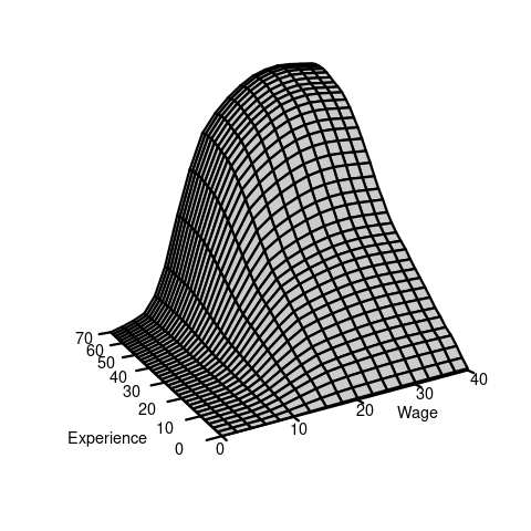
A bivariate random variable is a vector of two univariate random variables, e.g., (Y,Z), where Y is wage and Z is experience.
Bivariate distribution
The joint distribution function of a bivariate random variable (Y,Z) is
\begin{align*} F_{YZ}(a, b) &= P(Y \leq a, Z \leq b) \\ &= P(\{Y \leq a\} \cap \{ Z \leq b\}) \end{align*}
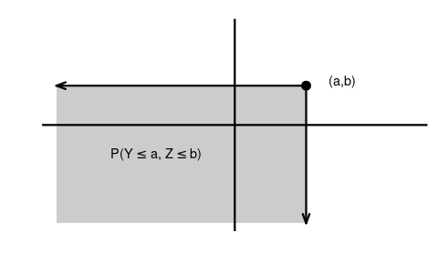
Probabilities can be calculated using a bivariate distribution function in the following way: P(Y \leq a, Z \leq b) = F_{YZ}(a, b)
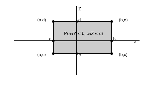
\begin{align*} &P(a < Y \leq b, c < Z \leq d) \\ &= F_{YZ}(b,d) - F_{YZ}(b,c) - F_{YZ}(a,d) + F_{YZ}(a,c) \end{align*}
Marginal distributions
The marginal distributions of Y and Z are \begin{align*} F_Y(a) &= P(Y \leq a) \\ &= P(Y \leq a, Z < \infty) \\ &= \lim_{b \to \infty} F_{YZ}(a,b) \end{align*} and \begin{align*} F_Z(b) &= P(Z \leq b) \\ &= P(Y < \infty, Z \leq b) \\ &= \lim_{a \to \infty} F_{YZ}(a,b). \end{align*}
While the above example shows a bivariate random variable containing two continuous random variables, we can also study discrete variables: Consider, for instance, the coin toss variable Y with P(Y=1) = 0.5 and P(Y=0) = 0.5, and let Z be a second coin toss with the same probabilities. X = (Y,Z) is a bivariate random variable where both entries are discrete random variables.
Since the two coin tosses are performed separately from each other, it is reasonable to assume that the probability that the first and second coin tosses show “heads” is 0.25, i.e., P(\{Y=1\} \cap \{Z=1\}) = 0.25. We would expect the following joint probabilities:
| Z=1 | Z=0 | any result | |
| Y=1 | 0.25 | 0.25 | 0.5 |
| Y=0 | 0.25 | 0.25 | 0.5 |
| any result | 0.5 | 0.5 | 1 |
The probabilities in the above table characterize the joint distribution of Y and Z. The table shows the values of the joint probability mass function: \pi_{YZ}(a,b) = \begin{cases} 0.25 & \text{if} \ a \in \{0,1\} \ \text{and} \ b \in \{0,1\} \\ 0 & \text{otherwise} \end{cases}
The joint CDF is: F_{YZ}(a, b) = \begin{cases} 0 & \text{if } a < 0 \text{ or } b < 0, \\ 0.25 & \text{if } 0 \leq a < 1 \text{ and } 0 \leq b < 1, \\ 0.5 & \text{if } 0 \leq a < 1 \text{ and } b \geq 1, \\ 0.5 & \text{if } a \geq 1 \text{ and } 0 \leq b < 1, \\ 1 & \text{if } a \geq 1 \text{ and } b \geq 1. \end{cases}
The marginal CDF of Y is: F_Y(a) = \begin{cases} 0 & \text{if } a < 0, \\ 0.5 & \text{if } 0 \leq a < 1, \\ 1 & \text{if } a \geq 1. \end{cases}
The marginal CDF of Z is: F_Z(b) = \begin{cases} 0 & \text{if } b < 0, \\ 0.5 & \text{if } 0 \leq b < 1, \\ 1 & \text{if } b \geq 1. \end{cases}
Another example are the random variables Y, a dummy variable for the event that the person has a high wage (more than 25 USD/hour), and Z, a dummy variable for the event that the same person has a university degree.
Similarly, X = (Y,Z) is a bivariate random variable consisting of two univariate Bernoulli variables. The joint probabilities might be as follows:
| Z=1 | Z=0 | any education | |
| Y=1 | 0.19 | 0.12 | 0.31 |
| Y=0 | 0.17 | 0.52 | 0.69 |
| any wage | 0.36 | 0.64 | 1 |
The joint probability mass function is \pi_{YZ}(a,b) = \begin{cases} 0.19 & \text{if} \ a=1, b=1, \\ 0.12 & \text{if} \ a=1, b=0, \\ 0.17 & \text{if} \ a=0, b=1, \\ 0.52 & \text{if} \ a=0, b=0, \\ 0 & \text{otherwise.} \end{cases}
The joint CDF is:
F_{YZ}(a, b) = \begin{cases} 0 & \text{if } a < 0 \text{ or } b < 0, \\ 0.52 & \text{if } 0 \leq a < 1 \text{ and } 0 \leq b < 1, \\ 0.69 & \text{if } 0 \leq a < 1 \text{ and } b \geq 1, \\ 0.64 & \text{if } a \geq 1 \text{ and } 0 \leq b < 1, \\ 1 & \text{if } a \geq 1 \text{ and } b \geq 1. \end{cases}
The marginal CDF of Y is: F_Y(a) = \begin{cases} 0 & \text{if } a < 0, \\ 0.69 & \text{if } 0 \leq a < 1, \\ 1 & \text{if } a \geq 1. \end{cases}
The marginal CDF of Z is: F_Z(b) = \begin{cases} 0 & \text{if } b < 0, \\ 0.64 & \text{if } 0 \leq b < 1, \\ 1 & \text{if } b \geq 1. \end{cases}
4.8 Independence
Two events A and B are independent if P(A \cap B) = P(A) P(B). For instance, in the bivariate random variable of Table 4.2 (two coin tosses), we have \begin{align*} P(Y=1, Z=1) &= 0.25 \\ &= 0.5 \cdot 0.5 \\ &= P(Y=1)P(Z=1). \end{align*} Hence, \{Y=1\} and \{Z=1\} are independent events. In the bivariate random variable of Table 4.3 (wage/education), we find \begin{align*} P(Y=1, Z=1) &= 0.19 \\ &\neq P(Y=1)P(Z=1) \\ &= 0.31 \cdot 0.36 \\ &= 0.1116. \end{align*} Therefore, the two events are not independent. In this case, the two random variables are dependent.
Independence
Y and Z are independent random variables if, for all a and b, the bivariate distribution function is the product of the marginal distribution functions: F_{YZ}(a,b) = F_Y(a) F_Z(b). If this property is not satisfied, we say that X and Y are dependent.
The random variables Y and Z of Table 4.2 are independent, and those of Table 4.3 are dependent.
4.9 Multivariate distributions
In statistics, we typically study multiple random variables simultaneously. We can collect n random variables Z_1, \ldots, Z_n in a n \times 1 random vector \boldsymbol Z = \begin{pmatrix} Z_1 \\ \vdots \\ Z_n \end{pmatrix}= (Z_1, \ldots, Z_n)'. We also call \boldsymbol Z a n-variate random variable.
For example, Z_1, \ldots, Z_n could represent n repeated coin tosses or the wage levels of the first n individuals interviewed.
Since \boldsymbol Z is a random vector, its outcome is also a vector, e.g., \{\boldsymbol Z = \boldsymbol b\} with \boldsymbol b = (b_1, \ldots, b_n)' \in \mathbb R^n. Events of the form \{\boldsymbol Z \leq \boldsymbol b\} mean that each component of the random vector \boldsymbol Z is smaller than the corresponding values of the vector \boldsymbol b, i.e. \{\boldsymbol Z \leq \boldsymbol b\} = \{Z_1 \leq b_1, \ldots, Z_n \leq b_n\}.
The concepts of the CDF and independence can be generalized to any n-variate random vector \boldsymbol Z = (Z_1, \ldots, Z_n)'. The joint CDF of \boldsymbol Z is \begin{align*} F_Z(\boldsymbol b) &= P(Z_1 \leq b_1, \ldots, Z_n \leq b_n) \\ &= P(\{Z_1 \leq b_1\} \cap \ldots \cap \{Z_n \leq b_n\}). \end{align*}
\boldsymbol Z has mutually independent entries if F_Z(\boldsymbol b) = \prod_{i=1}^n F_{Z_i}(b_i). That is, P(Z_1 \leq b_1, \ldots, Z_n \leq b_n) = P(Z_1 \leq b_1) \cdot \ldots \cdot P(Z_n \leq b_n).
4.10 IID sampling
In statistical analysis, a dataset \{\boldsymbol X_1, \ldots, \boldsymbol X_n\} that is drawn from some population F is called sample.
The CPS data are cross-sectional data, where n individuals are randomly selected from the US population and independently interviewed on k variables. The US data consists of n independently replicated random experiments.
i.i.d. sample / random sample
A collection of random vectors \{\boldsymbol X_1, \ldots, \boldsymbol X_n\} is i.i.d. (independent and identically distributed) if they are mutually independent and have the same distribution function F for all i \neq j.
An i.i.d. dataset or i.i.d. sample is also called a random sample. F is called population distribution or data-generating process (DGP).
Any transformed sample \{g(\boldsymbol X_1), \ldots, g(\boldsymbol X_n)\} of an i.i.d. sample \{\boldsymbol X_1, \ldots, \boldsymbol X_n\} is also an i.i.d. sample (g may be any function). For instance, if the wages of n interviewed individuals are i.i.d., then the log-wages are also i.i.d.
Sampling methods of obtaining economic datasets that may be considered as random sampling are:
-
Survey sampling
Examples: representative survey of randomly selected households from a list of residential addresses; online questionnaire to a random sample of recent customers -
Administrative records
Examples: data from a government agency database, Statistisches Bundesamt, ECB, etc. -
Direct observation
Collected data without experimental control and interactions with the subject. Example: monitoring customer behavior in a retail store -
Web scraping
Examples: collected house prices on real estate sites or hotel/electronics prices on booking.com/amazon, etc. -
Field experiment
To study the impact of a treatment or intervention on a treatment group compared with a control group. Example: testing the effectiveness of a new teaching method by implementing it in a selected group of schools and comparing results to other schools with traditional methods -
Laboratory experiment
Example: a controlled medical trial for a new drug
Examples of cross-sectional data sampling that may produce some dependence across observations are:
Stratified sampling
The population is first divided into homogenous subpopulations (strata), and a random sample is obtained from each stratum independently. Examples: divide companies into industry strata (manufacturing, technology, agriculture, etc.) and sample from each stratum; divide the population into income strata (low-income, middle-income, high-income).
The sample is independent within each stratum, but it is not between different strata. The strata are defined based on specific characteristics that may be correlated with the variables collected in the sample.Clustered sampling
Entire subpopulations are drawn. Example: new teaching methods are compared to traditional ones on the student level, where only certain classrooms are randomly selected, and all students in the selected classes are evaluated.
Within each cluster (classroom), the sample is dependent because of the shared environment and teacher’s performance, but between classrooms, it is independent.
Other types of data we often encounter in econometrics are time series data, panel data, or spatial data:
Time series data consists of observations collected at different points in time, such as stock prices, daily temperature measurements, or GDP figures. These observations are ordered and typically show temporal trends, seasonality, and autocorrelation.
Panel data involves observations collected on multiple entities (e.g., individuals, firms, countries) over multiple time periods.
Spatial data includes observations taken at different geographic locations, where values at nearby locations are often correlated.
Time series, panel, and spatial data cannot be considered a random sample given their temporal or geographic dependence.