8 Simulations

8.1 Consistent estimation

Recall the definitions of the bias, variance, and mean squared error (MSE) of an estimator \widehat \theta for a parameter \theta:

Bias: Bias(\widehat \theta) = E[\widehat \theta] - \theta
Variance: Var(\widehat \theta) = E[(\widehat \theta - E[\widehat \theta])^2]
MSE: MSE(\widehat \theta) = E[(\widehat \theta - \theta)^2]

These quantities are related by the equation: MSE(\widehat \theta) = Var(\widehat \theta) + Bias(\widehat \theta)^2. This relationship holds for any estimator and can be derived as follows: \begin{align*} MSE(\widehat \theta) &= E[(\widehat \theta - \theta)^2] \\ &= E[(\widehat \theta - E[\widehat \theta] + E[\widehat \theta] - \theta)^2] \\ &= E[(\widehat \theta - E[\widehat \theta])^2] + 2 E[(\widehat \theta - E[\widehat \theta])(E[\widehat \theta] - \theta)] + (E[\widehat \theta] - \theta)^2 \\ &= Var(\widehat \theta) + 2 (\underbrace{E[\widehat \theta] - E[\widehat \theta]}_{=0})(E[\widehat \theta] - \theta) + Bias(\widehat \theta)^2 \end{align*}

Recall that an estimator is consistent if it gets closer to the true parameter value as we collect more data. In mathematical terms, \widehat \theta is consistent for \theta if its MSE tends to zero as the sample size n \to \infty. This means both the bias and variance of \widehat \theta approach zero.

To understand the consistency properties of an estimator \widehat \theta, an alternative to mathematical proofs is to conduct a Monte Carlo simulation. These simulations are useful for studying the sampling distribution of a statistic in a controlled environment where the true data-generating population distribution is known. They allow us to compare the biases and MSEs of different estimators for different sample sizes.

While mathematical proofs establish theoretical properties of estimators, Monte Carlo simulations show us how these estimators actually behave with real, finite samples. These simulations let us examine an estimator’s performance under different conditions and sample sizes, and help us develop statistical intuition.

The idea is to use computer-generated pseudorandom numbers to create artificial datasets of sample size n. We apply the estimator of interest to each dataset, which generates random draws from the distribution of the estimator. By repeating this procedure independently B times, we obtain an i.i.d. sample of size B from the distribution of the estimator, known as a Monte Carlo sample. From this sample, we can compute empirical estimates of quantities like bias, variance, and MSE.

8.2 Set up

To set up the Monte Carlo simulation for \widehat \theta, we need to specify

Estimator (\widehat \theta): The estimator of interest.
Population distribution (F): The specific distribution from which we sample our data.
Parameter value (\theta): The particular value of the parameter of F that we aim to estimate.
Sample size (n): The number of observations in each simulated dataset.
Sampling scheme: Typically independent and identically distributed (i.i.d.), but it could also involve dependence (e.g., in time series data).
Number of repetitions (B): The number of times the simulation is repeated to generate a Monte Carlo sample.

For example, if we are interested in the MSE of the sample mean of 100 i.i.d. coin flips, we set:

\widehat \theta = \overline Y (the sample mean),
F as the Bernoulli distribution with P(Y=1) = 0.5,
\theta = E[Y] = 0.5 (the population mean),
n=100,
an i.i.d. sampling scheme,
a large number of repetitions, such as B=10000.

8.3 Monte Carlo algorithm

The Monte Carlo simulation is performed as follows:

Using the specified sampling scheme, draw a sample \{\boldsymbol X_1, \ldots, \boldsymbol X_n \} of size n from F using the computer’s random number generator. Evaluate the estimator \widehat \theta from \{\boldsymbol X_1, \ldots, \boldsymbol X_n\}.
Repeat step 1 of the experiment B times and collect the estimates in the Monte Carlo sample \widehat \theta_{mc} = \{\widehat \theta_1, \ldots, \widehat \theta_B \}.
Estimate the features of interest from the Monte Carlo sample:
- Mean: \widehat \mu_{mc} = \frac{1}{B} \sum_{i=1}^B \widehat \theta_i.
- Bias: \widehat{Bias}(\widehat \theta_{mc}) = \widehat \mu_{mc} - \theta
- Variance: \widehat{Var}(\widehat \theta_{mc}) = \frac{1}{B-1} \sum_{i=1}^B (\widehat \theta_i - \widehat \mu_{mc})^2
- MSE: \widehat{MSE}(\widehat \theta_{mc}) = \widehat{Var}(\widehat \theta_{mc}) + \widehat{Bias}(\widehat \theta_{mc})^2

8.4 Sample mean of coin flips

Let’s conduct a Monte Carlo simulation for the sample mean of coin flips.

set.seed(1)  # Set seed for reproducibility

# Function to generate a random sample and compute its sample mean
getMCsample = function(n) {
  # Generate an i.i.d. Bernoulli sample of size n with probability 0.5
  X = rbinom(n, size = 1, prob = 0.5)
  # Compute and return the sample mean of X
  mean(X)
}

# True parameter value (population mean) of the Bernoulli distribution
theta = 0.5

# Number of Monte Carlo repetitions
B = 1000

# Function to perform Monte Carlo simulation and calculate Bias, Variance, and MSE for a given sample size
simulate_bias_variance_mse = function(n) {
  # Generate a Monte Carlo sample of B sample means
  MCsample = replicate(B, getMCsample(n))
  # Calculate Bias, Variance, and MSE
  Bias = mean(MCsample) - theta
  Variance = var(MCsample)
  MSE = Variance + Bias^2
  # Return the results as a vector
  c(Bias, Variance, MSE)
}

# Run the simulation for different sample sizes and store results
result10 = simulate_bias_variance_mse(10)
result20 = simulate_bias_variance_mse(20)
result50 = simulate_bias_variance_mse(50)
results = cbind(result10, result20, result50)

# Assign names to columns and rows for clarity in the output
colnames(results) = c("n=10", "n=20", "n=50")
rownames(results) = c("Bias", "Variance", "MSE")

# Display the results
results

                n=10        n=20        n=50
Bias     -0.00470000 -0.00370000 0.004740000
Variance  0.02605396  0.01272403 0.004631364
MSE       0.02607605  0.01273772 0.004653831

This output shows how the bias, variance, and MSE decrease as the sample size increases, which illustrates the consistency of the estimator.

8.5 Linear and nonlinear regression

Let’s use Monte Carlo simulations to study the consistency properties of the OLS estimator in a simple linear regression model. We expect \widehat \beta_2 to be a consistent estimator for \beta_2 in the following regression model: Y_i = \beta_1 + \beta_2 Z_i + u_i, \quad E[u_i|Z_i] = 0, \tag{8.1} provided (A2)–(A4) hold true. In this case, \widehat \beta_2 is \widehat \beta_2 = \frac{\widehat \sigma_{YZ}}{\widehat \sigma_Z^2}. \tag{8.2}

However, the true relationship between Y and Z might be nonlinear such that the true model has the form Y_i = \beta_1 + \beta_2 Z_i + \beta_3 Z_i^2 + \beta_4 Z_i^3 + v_i, \quad E[v_i|Z_i] = 0. \tag{8.3} Note that u_i = \beta_3 Z_i^2 + \beta_4 Z_i^3 + v_i. Hence, if \beta_3 \neq 0, then \begin{align*} E[u_i|Z_i] &= E[\beta_3 Z_i^2 + \beta_4 Z_i^3 + v_i|Z_i] \\ &= \beta_3 Z_i^2 + \beta_4 Z_i^3 + E[v_i|Z_i] \\ &= \beta_3 Z_i^2 + \beta_4 Z_i^3 \neq 0, \end{align*} and the simple model from Equation 8.1 cannot be true. This means the error term contains systematic patterns related to Z_i, which violates a key assumption (A1) of linear regression.

In this case, using \widehat \beta_2 from Equation 8.2 to estimate \beta_2 from Equation 8.3 will lead to a biased estimate.

Let’s simulate data from models Equation 8.1 and Equation 8.3 where:

Z_i, u_i, v_i are i.i.d. and \mathcal N(0,1) (standard normal distribution)
n=100
\beta_1 = 1, \beta_2 = 2, \beta_3 = -3, \beta_4 = -1

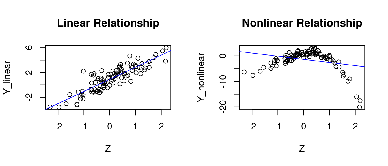
set.seed(123)  # For reproducibility

# Parameters
beta1 = 1
beta2 = 2
beta3 = -3
beta4 = -1
n = 100

# Data generation
Z = rnorm(n)
Y_linear = beta1 + beta2 * Z + rnorm(n)
Y_nonlinear = beta1 + beta2 * Z + beta3 * Z^2 + beta4 * Z^3 + rnorm(n)

# Linear Case Plot with Regression Line
par(mfrow = c(1, 2))
plot(Z, Y_linear, main = "Linear Relationship")
fit1 = lm(Y_linear ~ Z) # fit simple linear model
abline(fit1, col = "blue")  # Add linear regression line

# Nonlinear Case Plot with Regression Line
plot(Z, Y_nonlinear, main = "Nonlinear Relationship")
fit2 = lm(Y_nonlinear ~ Z) # fit simple linear model without Z^2
abline(fit2, col = "blue")  # Add linear regression line

In the left plot, the model is correctly specified, i.e., E[u_i|Z_i] = 0 holds. In the right plot, the model is misspecified, i.e., E[u_i|Z_i] \neq 0.

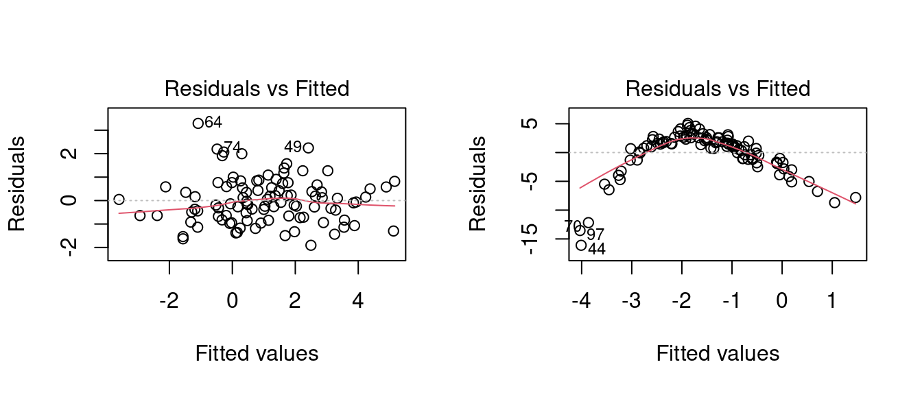
This becomes also evident in the residuals versus fitted values plots. The residuals serve as proxies for the unknown error terms, while the fitted values \widehat Y_i = \boldsymbol X_i'\widehat{\boldsymbol \beta} provide a one-dimensional summary of all regressors.

Residuals that are equally spread around a horizontal line without distinct patterns, as shown in the left plot below, indicate a correctly specified linear model. When the size or sign of the residuals systematically depends on the fitted values, as in the right plot below, this suggests hidden nonlinear relationships between the response and predictors that the model fails to capture.

## Diagnostics plot
par(mfrow = c(1, 2))
plot(fit1, which = 1)
plot(fit2, which = 1)

The red solid line indicates a local scatterplot smoother, which is a smooth locally weighted line through the points on the scatterplot to visualize the general pattern of the data.

8.5.1 Simulation of the linear case

To assess the statistical properties of our estimator, we examine how accurately \widehat \beta_2 from Equation 8.2 estimates the true parameter \beta_2 in the correctly specified model Equation 8.1.

set.seed(1)  # Set seed for reproducibility

# True parameter values
beta1 = 1
beta2 = 2

# Generate a random sample and compute OLS coefficient beta2-hat
getMCsample = function(n) {
  # Data generation
  Z = rnorm(n)
  Y_linear = beta1 + beta2 * Z + rnorm(n)
  fit1 = lm(Y_linear ~ Z) # fit simple linear model
  # Compute and return beta2-hat
  fit1$coefficients[2]
}

# Number of Monte Carlo repetitions
B = 1000

# Function to perform Monte Carlo simulation and calculate Bias, Variance, and MSE for a given sample size
simulate_bias_variance_mse = function(n) {
  # Generate a Monte Carlo sample of B sample means
  MCsample = replicate(B, getMCsample(n))
  # Calculate Bias, Variance, and MSE
  Bias = mean(MCsample) - beta2
  Variance = var(MCsample)
  MSE = Variance + Bias^2
  # Return the results as a vector
  c(Bias, Variance, MSE)
}

# Run the simulation for different sample sizes and store results
result10 = simulate_bias_variance_mse(10)
result20 = simulate_bias_variance_mse(20)
result50 = simulate_bias_variance_mse(50)
results = cbind(result10, result20, result50)

# Assign names to columns and rows for clarity in the output
colnames(results) = c("n=10", "n=20", "n=50")
rownames(results) = c("Bias", "Variance", "MSE")

# Display the results
results

              n=10         n=20         n=50
Bias     0.0155187 -0.003998293 -0.001679989
Variance 0.1468236  0.056849539  0.021480276
MSE      0.1470645  0.056865525  0.021483098

The bias of \widehat{\beta}_2 is close to zero for all sample sizes.
The variance decreases as n increases.
The MSE decreases with larger n, which indicates that \widehat{\beta}_2 is a consistent estimator when the model is correctly specified.

8.5.2 Simulation of the nonlinear case

We now examine how the OLS estimator \widehat \beta_2 from the linear model Equation 8.2 performs when the true data generating process contains nonlinear terms, as specified in Equation 8.3. This allows us to quantify the bias that arises from omitting the nonlinear terms.

set.seed(1)  # Set seed for reproducibility

# True parameter values
beta1 = 1
beta2 = 2
beta3 = -3
beta4 = -1

# Generate a random sample and compute OLS coefficient beta2-hat
getMCsample = function(n) {
  # Data generation
  Z = rnorm(n)
  Y_nonlinear = beta1 + beta2 * Z + beta3 * Z^2 + beta4 * Z^3 + rnorm(n)
  fit2 = lm(Y_nonlinear ~ Z) # fit simple linear model without Z^2
  # Compute and return beta2-hat
  fit2$coefficients[2]
}

# Number of Monte Carlo repetitions
B = 1000

# Function to perform Monte Carlo simulation and calculate Bias, Variance, and MSE for a given sample size
simulate_bias_variance_mse = function(n) {
  # Generate a Monte Carlo sample of B sample means
  MCsample = replicate(B, getMCsample(n))
  # Calculate Bias, Variance, and MSE
  Bias = mean(MCsample) - beta2
  Variance = var(MCsample)
  MSE = Variance + Bias^2
  # Return the results as a vector
  c(Bias, Variance, MSE)
}

# Run the simulation for different sample sizes and store results
result10 = simulate_bias_variance_mse(10)
result20 = simulate_bias_variance_mse(20)
result50 = simulate_bias_variance_mse(50)
results = cbind(result10, result20, result50)

# Assign names to columns and rows for clarity in the output
colnames(results) = c("n=10", "n=20", "n=50")
rownames(results) = c("Bias", "Variance", "MSE")

# Display the results
results

              n=10      n=20      n=50
Bias     -2.514799 -2.653668 -2.844885
Variance  8.606104  5.340871  2.118467
MSE      14.930317 12.382827 10.211839

The bias of \widehat{\beta}_2 is substantial and does not decrease with larger n.
The variance decreases with larger n, but the MSE remains high due to the large bias.
This demonstrates that omitting the relevant nonlinear terms (Z_i^2 and Z_i^3) leads to a biased and inconsistent estimator of \beta_2 when the true model is nonlinear.

8.6 R-codes

statistics-sec08.R