5 Expectation
The expectation or expected value is the most important measure of the central tendency of a distribution. It gives you the average value you can expect to get if you repeat the random experiment multiple times. We define the expectation first for discrete random variables, then continuous random variables, and finally give a unified definition for all random variables.
5.1 Discrete random variables
Recall that a discrete random variable Y is a variable that can take on a countable number of distinct values. Each possible value a has an associated probability \pi(a)=P(Y=a), known as the probability mass function (PMF).
The support \mathcal Y of Y is the set of all values that Y can take with non-zero probability: \mathcal{Y} = \{ a \in \mathbb{R} : \pi(a) > 0 \}. The total probability sums to 1: \sum_{a \in \mathcal Y} \pi(a)= 1.
The expectation or expected value of a discrete random variable Y with PMF \pi(\cdot) and support \mathcal Y is defined as E[Y] = \sum_{u \in \mathcal Y} u \pi(u). \tag{5.1}
The expected value of the variable education from the previous section is calculated by summing over all possible values: \begin{align*} E[Y] &= 4\cdot\pi(4) + 10\cdot\pi(10) + 12\cdot \pi(12) \\ &\phantom{=} + 13\cdot\pi(13) + 14\cdot\pi(14) + 16\cdot \pi(16) \\ &\phantom{=} + 18 \cdot \pi(18) + 21 \cdot \pi(21) = 14.117 \end{align*}
A binary or Bernoulli random variable Y takes on only two possible values: 0 and 1. The support is \mathcal Y = \{0,1\}. The probabilities are
- \pi(1) = P(Y=1) = p
- \pi(0) = P(Y=0) = 1-p
for some p \in (0,1). The expected value of Y is: \begin{align*} E[Y] &=0\cdot\pi(0) + 1\cdot\pi(1) \\ &= 0 \cdot(1-p) + 1 \cdot p \\ &= p. \end{align*} For the variable coin, the probability of heads is p=0.5 and the expected value is E[Y] = p = 0.5.
5.2 Continuous random variables
For discrete random variables, both the PMF and the CDF characterize the distribution. For continuous random variables, the PMF concept does not apply because the probability of any specific point is zero. The continuous counterpart of the PMF is the density function:
Probability density function
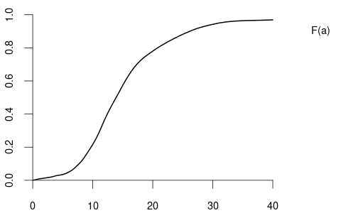
The probability density function (PDF) or simply density function of a continuous random variable Y with CDF F(a) is a function f(a) that satisfies F(a) = \int_{-\infty}^a f(u) \ \text{d}u If the CDF is differentiable, the density f(a) is its derivative: f(a) = \frac{d}{da} F(a).
Properties of a PDF:
f(a) \geq 0 for all a \in \mathbb R
\int_{-\infty}^\infty f(u) \ \text{d}u = 1
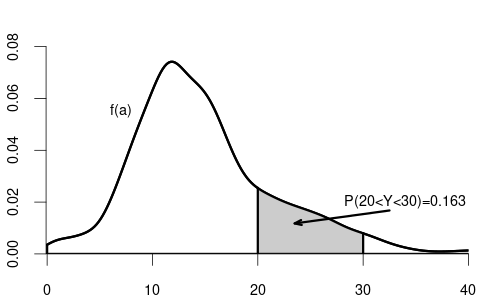
Probability rule for the PDF: P(a < Y < b) = \int_a^b f(u) \ \text{d} u = F(b) - F(a)
The expectation or expected value of a continuous random variable Y with PDF f(\cdot) is E[Y] = \int_{-\infty}^\infty u f(u) \ \text{d}u. \tag{5.2}
The uniform distribution on the unit interval [0,1] has the PDF f(u) = \begin{cases} 1 & \text{if} \ u \in[0,1], \\ 0 & \text{otherwise,} \end{cases} \tag{5.3} and the expected value of a uniformly distributed random variable Y is E[Y] = \int_{-\infty}^\infty u f(u) \ \text{d} u = \int_{0}^1 u \ \text{d} u = \frac{1}{2} u^2 \ \bigg|_0^1= \frac{1}{2}.
5.3 Unified definition of the expected value
The expected value of a random variable Y can be defined in a unified way that applies to both discrete and continuous cases by using its CDF F(u): E[Y] = \int_{-\infty}^\infty u \ \text{d}F(u). \tag{5.4}
This integral, known as the Riemann-Stieltjes integral, generalizes the concept of integration to include functions that may not be smooth or differentiable everywhere.
For a continuous random variable with PDF f(u), the CDF F(u) is smooth and differentiable. The relationship between the CDF and the PDF is: \text{d}F(u)=f(u) \ \text{d}u. Substituting this into our unified definition gives: \begin{align*} E[Y] &= \int_{-\infty}^\infty u \ \text{d}F(u) \\ &= \int_{-\infty}^\infty u f(u) \ \text{d}u, \end{align*} which matches the standard definition of the expected value for continuous random variables as in Equation 5.2.
For a discrete random variable, the CDF F(u) is a step function that increases in jumps at the possible values u \in \mathcal Y that Y can take. The “change” or jump in the CDF at each u \in \mathcal Y is: \Delta F(u) = F(u) - F(u^-) = P(Y=u) = \pi(u), where F(u^-) is the value of F(u) just before u, and \pi(u) is the PMF of Y.
Integrating with respect to F(u) simplifies to summing over these jumps: \begin{align*} E[Y] &= \int_{-\infty}^\infty u \ \text{d}F(u) \\ &= \sum_{u \in \mathcal Y} u \ \Delta F(u) \\ &= \sum_{u \in \mathcal Y} u \pi(u), \end{align*} which aligns with the standard definition of the expected value for discrete random variables as in Equation 5.1.
The unified definition E[Y]= \int_{-\infty}^\infty u \ \text{d}F(u) allows us to treat all types of random variables consistently, whether the variable is discrete, continuous, or a mixture of both. It can also handle non-standard cases such as distributions with CDFs that are not differentiable everywhere.
5.4 Transformed variables
We often transform random variables by taking, for instance, squares Y^2 or logs \log(Y). For any transformation function g(\cdot), the expectation of the transformed random variable g(Y) is E[g(Y)] = \int_{-\infty}^\infty g(u) \ \text{d}F(u), where F(u) is the CDF of Y. As discussed in Section 5.3 for the different cases, \text{d}F(u) can be replaced by the PMF or the PDF, i.e., \int_{-\infty}^\infty g(u) \ \text{d}F(u) = \begin{cases} \sum_{u \in \mathcal Y} g(u) \pi(u) & \text{if} \ Y \ \text{is discrete,} \\ \int_{-\infty}^\infty g(u) f(u)\text{d}u & \text{if} \ Y \ \text{is continuous.} \end{cases}
For instance, if we take the coin variable Y and consider the transformed random variable \log(Y+1), the expected value is E[\log(Y+1)] = \log(1) \cdot \frac{1}{2} + \log(2) \cdot \frac{1}{2} = \frac{\log(2)}{2} We can define the population counterparts of the sample moments and their centralized and standardized versions:
- r-th moment of Y: E[Y^r] = \int_{-\infty}^\infty u^r \ \text{d}F(u)
- r-th central moment: E[(Y-E[Y])^r] = \int_{-\infty}^\infty (u - E[Y])^r \ \text{d}F(u)
- Variance (2nd central moment): Var[Y] = E[(Y-E[Y])^2] = \int_{-\infty}^\infty (u - E[Y])^2 \ \text{d}F(u)
- Standard deviation: sd(Y) = \sqrt{Var[Y]}
- r-th standardized moment: E \bigg[ \Big(\frac{Y-E[Y]}{sd(Y)}\Big)^r \bigg] = \int_{-\infty}^\infty \Big(\frac{u-E[Y]}{sd(Y)}\Big)^r \ \text{d}F(u)
- Skewness (3rd standardized moment): skew(Y) = E \bigg[ \Big(\frac{Y-E[Y]}{sd(Y)}\Big)^3 \bigg]
- Kurtosis (4th standardized moment): kurt(Y) = E \bigg[ \Big(\frac{Y-E[Y]}{sd(Y)}\Big)^4 \bigg]
5.5 Linearity of the expected value
The expected value is a linear function. For any a,b \in \mathbb R, we have E[aY + b] = a E[Y] + b. For the variance, the following rule applies: Var[aY + b] = a^2 Var[Y].
For any two random variables Y and Z, we have E[aY + bZ] = aE[Y] + bE[Z]. A similar result for the variance does not hold in general. However, if Y and Z are independent random variables, we have Var[aY + bZ] = a^2 Var[Y] + b^2 Var[Z]. \tag{5.5}
5.6 Parameters and estimators
A parameter \theta is a feature (function) of the population distribution F of some random variable Y. The expectation, variance, skewness, and kurtosis are parameters.
A statistic is a function of a sample Y_1, \ldots, Y_n. An estimator \widehat \theta for \theta is a statistic intended as a guess about \theta. It is a function of the random variables Y_1, \ldots, Y_n and, therefore, a random variable as well. The sample mean, sample variance, sample skewness and sample kurtosis are estimators. When an estimator \widehat \theta is calculated in a specific realized sample, we call \widehat \theta an estimate.
5.7 Estimation of the mean
The expected value E[Y] is also called population mean because it is the population counterpart of the sample mean \overline Y = \frac{1}{n} \sum_{i=1}^n Y_i, where the sample Y_1, \ldots, Y_n is identically distributed and has the same distribution as Y. In particular, we have: E[Y_1] = \ldots = E[Y_n] = E[Y].
The true population mean E[Y] is unknown in practice, but we can use the sample mean \overline Y to estimate it. The sample mean is an unbiased estimator for the population mean because E[\overline Y] = \frac{1}{n} \sum_{i=1}^n E[Y_i] = \frac{1}{n} \sum_{i=1}^n E[Y] = E[Y]. The bias of an estimator is the expected value of the estimator minus the parameter to be estimated. The bias of the sample mean is zero: Bias[\overline Y] = E[\overline Y] - E[Y] = E[Y] - E[Y] = 0. When repeating random experiments and computing sample means, we can expect the sample means to be distributed around the true population mean, with the population mean at the center of this distribution.
To assess how large the spread around the true population mean is, we can compute the variance: Var[\overline Y] = \frac{1}{n^2} Var\bigg[ \sum_{i=1}^n Y_i \bigg] To simplify this term further, let’s assume that the sample is i.i.d. (independent and identically distributed), i.e. the observations are randomly sampled from the population. Then, we can apply Equation 5.5: Var\bigg[ \sum_{i=1}^n Y_i \bigg] = \sum_{i=1}^n Var[Y_i]. By the identical distribution of the sample, we have Var[Y_1] = \ldots = Var[Y_n] = Var[Y]. Therefore, the variance of the sample mean becomes: Var[\overline Y] = \frac{1}{n^2} \sum_{i=1}^n Var[Y_i] = \frac{1}{n^2} \sum_{i=1}^n Var[Y] = \frac{Var[Y]}{n}. The spread of sample means around the true mean becomes smaller, the larger the sample size n is. The more observations we have, the more precisely the sample mean can estimate the true population mean.
5.8 Consistency
Good estimators get closer and closer to the true parameter being estimated as the sample size n increases, eventually returning the true parameter value in a hypothetically infinitely large sample. This property is called consistency.
Consistency
An estimator \widehat \theta is consistent for a true parameter \theta if, for any \epsilon > 0, P(|\widehat \theta - \theta| > \epsilon) \to 0 \qquad \text{as} \ n \to \infty. Equivalently, consistency can be defined by the complementary event: P(|\widehat \theta - \theta| \leq \epsilon) \to 1 \qquad \text{as} \ n \to \infty. If \widehat \theta is consistent, we say it converges in probability to \theta, denoted by \widehat \theta \overset{p} \to \theta \qquad \text{as} \ n \to \infty.
If an estimator \widehat \theta is a continuous random variable, it will almost never reach exactly the true parameter value because point probabilities are zero: P(\widehat \theta = \theta) = 0.
However, the larger the sample size, the higher should be the probability that \widehat \theta is close to the true value \theta. Consistency means that, if we fix some small precision value \epsilon > 0, then, P(|\widehat \theta - \theta| \leq \epsilon) = P( \theta - \epsilon \leq \widehat \theta \leq \theta + \epsilon) should increase in the sample size n and eventually reach 1.
An estimator is called inconsistent if it is not consistent. An inconsistent estimator is practically useless and leads to false inference. Therefore, it is important to verify that your estimator is consistent.
To show whether an estimator is consistent, we can check the sufficient condition for consistency:
Sufficient condition for consistency
Let \widehat \theta be an estimator for some parameter \theta. The bias of \widehat \theta is Bias[\widehat \theta] = E[\widehat \theta] - \theta.
If the bias and the variance of \widehat \theta tends to zero for large sample sizes, i.e., if
- Bias[\widehat \theta] \rightarrow 0 (as n \to \infty),
- Var[\widehat \theta] \rightarrow 0 (as n \to \infty),
then \widehat \theta is consistent for \theta.
The reason for this sufficient condition is the fact that P(|\widehat \theta - \theta| > \epsilon) \leq Var[\widehat \theta] + Bias[\widehat \theta]^2, which follows from Markov’s inequality.
5.9 Law of large numbers
The sample mean \overline Y of an i.i.d. sample is consistent for the population mean E[Y] because
- Bias[\overline Y] = 0 for all n;
- Var[\overline Y] = Var[Y]/n \to 0, as n \to \infty, provided Var[Y] < \infty.
The consistency result of the sample mean is also known as the law of large numbers (LLN): \overline Y \overset{p} \to E[Y] \qquad \text{as} \ n \to \infty. Below is an interactive Shiny app to visualize the law of large numbers using simulated data for different sample sizes and different distributions.
5.10 Heavy tails
The sample mean of i.i.d. samples from most distributions is consistent. However, there are some exceptional cases where consistency fails. For instance, the simple Pareto distribution has the PDF f(u) = \begin{cases} \frac{1}{u^2} & \text{if} \ u > 1, \\ 0 & \text{if} \ u \leq 1, \end{cases} and the expected value is E[X] = \int_{-\infty}^\infty u f(u) \ \text{d}u = \int_{1}^\infty \frac{1}{u} \ \text{d}u = \log(u)|_1^\infty = \infty. The population mean is infinity, so the sample mean cannot converge and is inconsistent. The game of chance from the St. Petersburg paradox (see https://en.wikipedia.org/wiki/St._Petersburg_paradox) is an example of a discrete random variable with infinite expectation.
Another example is the t-distribution with 1 degree of freedom, also denoted as t_1 or Cauchy distribution, which has the PDF f(u) = \frac{1}{\pi (1+u^2)}. The lack of consistency of the sample mean from a t_1 distribution is visualized in the shiny application above.
The Pareto, St. Petersburg, and Cauchy distributions have infinite population mean, and the sample mean of observations from these distributions is inconsistent. These are distributions that produce huge outliers.
There are other distributions that have a finite mean but an infinite variance, skewness, or kurtosis.
For instance, the t_2 distribution has a finite mean but an infinite variance. The t_3 distribution has a finite variance but an infinite skewness. The t_4 distribution has a finite skewness but an infinite kurtosis.
If Y is t_m-distributed (t-distribution with m degrees of freedom), then E[Y], E[Y^2], \ldots, E[Y^{m-1}] < \infty but E[Y^m] = E[Y^{m+1}] = \ldots = \infty.
Random variables with infinite first four moments have a so-called heavy-tailed distribution and may produce huge outliers. Many statistical procedures are only valid if the underlying distribution is not heavy-tailed.
5.11 Estimation of the variance
Consider an i.i.d. sample Y_1, \ldots, Y_n from some population distribution with population mean \mu = E[Y] and population variance \sigma^2 = Var[Y] < \infty.
We introduced two sample cointerparts of \sigma^2: the sample variance \widehat \sigma_Y^2 = \frac{1}{n} \sum_{i=1}^n (Y_i - \overline Y)^2, and the adjusted sample variance s_Y^2 = \frac{1}{n-1} \sum_{i=1}^n (Y_i - \overline Y)^2 = \frac{n}{n-1} \widehat \sigma_Y^2.
The sample variance can be decomposed as \begin{align*} \widehat \sigma_Y^2 &= \frac{1}{n} \sum_{i=1}^n (Y_i - \overline Y)^2 =\frac{1}{n} \sum_{i=1}^n (Y_i - \mu + \mu - \overline Y)^2 \\ &= \frac{1}{n} \sum_{i=1}^n(Y_i - \mu)^2 + \frac{2}{n} \sum_{i=1}^n (Y_i - \mu)(\mu - \overline Y) + \frac{1}{n} \sum_{i=1}^n (\mu - \overline Y)^2 \\ &= \frac{1}{n} \sum_{i=1}^n(Y_i - \mu)^2 - 2(\overline Y - \mu)^2 + (\overline Y - \mu)^2 \\ &= \frac{1}{n} \sum_{i=1}^n(Y_i - \mu)^2 - (\overline Y - \mu)^2 \end{align*} The mean of \widehat \sigma_Y^2 is \begin{align*} E[\widehat \sigma_Y^2] &= \frac{1}{n} \sum_{i=1}^n E[(Y_i - \mu)^2] - E[(\overline Y - \mu)^2] = \frac{1}{n} \sum_{i=1}^n Var[Y_i] - Var[\overline Y] \\ &= \sigma^2 - \frac{\sigma^2}{n} = \frac{n-1}{n} \sigma^2, \end{align*} where we used the fact that Var[\overline Y] = \sigma^2/n.
The sample variance is downward biased: \begin{align*} Bias[\widehat \sigma_Y^2] = E[\widehat \sigma_Y^2] - \sigma^2 = \frac{n-1}{n} \sigma^2 - \sigma^2 = -\frac{\sigma^2}{n}. \end{align*}
On the other hand, the adjusted sample variance is unbiased:
\begin{align*}
Bias[s_Y^2] = E[s_Y^2] - \sigma^2 = \frac{n}{n-1}E[\widehat \sigma_Y^2] - \sigma^2 = \sigma^2 - \sigma^2 = 0
\end{align*}
The variance of the sample variance can be computed as Var[\widehat \sigma_Y^2] = \frac{\sigma^4}{n} \Big( kurt - \frac{n-3}{n-1} \Big) \frac{(n-1)^2}{n^2}, while the variance of the adjusted sample variance is Var[s_Y^2] = \frac{\sigma^4}{n} \Big( kurt - \frac{n-3}{n-1} \Big). As long as the kurtosis of the underlying distribution is finite, the sufficient conditions for consistency are satisfied as the bias and variance tend to zero as n \to \infty. The adjusted sample variance is unbiased for any n. The sample variance is biased for fixed n but asymptotically unbiased as the bias tends to zero for large n. The sample variance and the adjusted sample variance are consistent for the variance if the sample is i.i.d. and the distribution is not heavy-tailed.
5.12 Bias-variance tradeoff
From a bias perspective, adjusted sample variance s_Y^2 is preferred over \widehat \sigma^2_Y because s_Y^2 is unbiased. However, from a variance perspective, \widehat \sigma^2_Y is preferred due to its smaller variance. Traditionally, the emphasis on unbiasedness has led to a preference for \widehat \sigma^2_Y, even at the cost of a higher variance.
A more modern approach balances bias and variance, known as the bias-variance tradeoff, by selecting an estimator that minimizes the mean squared error (MSE): MSE(\widehat \theta) = E[(\widehat \theta - \theta)^2] = Var[\widehat \theta] + Bias[\widehat \theta]^2. For the variance estimators, the MSEs are MSE[\widehat \sigma_Y^2] = Var[\widehat \sigma_Y^2] + Bias[\widehat \sigma_Y^2]^2 = \frac{\sigma^4}{n} \bigg[ \Big( kurt - \frac{n-3}{n-1} \Big) \frac{(n-1)^2}{n^2} + \frac{1}{n} \bigg] and MSE[s_Y^2] = Var[s_Y^2] = \frac{\sigma^4}{n} \Big( kurt - \frac{n-3}{n-1} \Big). Since s_Y^2 is unbiased, its MSE equals its variance.
It is not possible to universally determine which estimator has a lower MSE because this depends on the population kurtosis (kurt) of the underlying distribution. However, it can be shown that for all distributions with kurt \geq 1.5, the relation MSE[s_Y^2] > MSE[\widehat \sigma_Y^2] holds, which implies that \widehat \sigma_Y^2 is preferred based on the bias-variance tradeoff for all moderately tailed distributions.
To give an indication of typical kurtosis values:
- Symmetric Bernoulli distribution with P(Y=0) = P(Y=1) = 0.5: kurtosis of 1 (light-tailed).
- Uniform distribution (see Equation 5.3): kurtosis of 1.8 (moderately light-tailed).
- Normal distribution: kurtosis of 3 (moderately tailed).
- t_5 distribution: kurtosis of 9 (moderately heavy-tailed).
- t_4 distribution: infinite kurtosis (heavy-tailed).
Therefore, according to the bias-variance tradeoff, the adjusted sample variance s_Y^2 is preferred only for extremely light-tailed distributions, while \widehat \sigma_Y^2 is preferred in cases with moderate or higher kurtosis.
In practice, especially with larger samples, the difference between s_Y^2 and \widehat \sigma_Y^2 becomes negligible, and either estimator is generally acceptable. Therefore, the discussion about a better variance estimator is a bit nitpicky and not of much practical relevance.
However, for instance in high-dimensional regression problems with near multicollinearity (k \approx n), the bias-variance tradeoff is crucial. In such cases, biased but low-variance estimators like ridge or lasso (shrinkage estimators) are often preferred over ordinary least squares (OLS).