6 Covariance
6.1 Expectation of bivariate random variables
We often are interested in expected values of functions involving two random variables, such as the cross-moment E[YZ] for variables Y and Z.
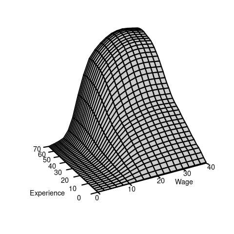
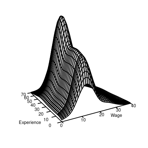
If F(a,b) is the joint CDF of (Y,Z), then the cross-moment is defined as: E[YZ] = \int_{-\infty}^\infty \int_{-\infty}^\infty ab \ \text{d}F(a,b). \tag{6.1} If Y and Z are continuous and F(a,b) is differentiable, the joint probability density function (PDF) of (Y,Z): f(a,b) = \frac{\partial^2}{\partial a \partial b} F(a,b). This allows us to write the differential of the CDF as \text{d}F(a,b) = f(a,b) \ \text{d} a \ \text{d}b, and the cross-moment becomes: E[YZ] = \int_{-\infty}^\infty \int_{-\infty}^\infty ab \ \text{d}F(a,b) = \int_{-\infty}^\infty \int_{-\infty}^\infty ab f(a,b) \ \text{d} a \ \text{d}b. In the wage and experience example, we have the following joint CDF and joint PDF:
If Y and Z are discrete with joint PMF \pi(a,b) and support \mathcal Y, the cross moment is E[YZ] = \int_{-\infty}^\infty \int_{-\infty}^\infty ab \ \text{d}F(a,b) = \sum_{a \in \mathcal Y} \sum_{b \in \mathcal Y} ab \ \pi(a,b). If one variable is discrete and the other is continuous, the expectation involves a mixture of summation and integration.
In general, the expected value of any real valued function g(Y,Z) is given by E[g(X,Y)] = \int_{-\infty}^\infty \int_{-\infty}^\infty g(a,b) \ \text{d}F(a,b).
6.2 Covariance and correlation
The covariance of Y and Z is defined as:
Cov(Y,Z) = E[(Y- E[Y])(Z-E[Z])] = E[YZ] - E[Y]E[Z].
The covariance of Y with itself is the variance:
Cov(Y,Y) = Var[Y].
The variance of the sum of two random variables depends on the covariance:
Var[Y+Z] = Var[Y] + 2 Cov(Y,Z) + Var[Z]
The correlation of Y and Z is
Corr(Y,Z) = \frac{Cov(Y,Z)}{sd(Y) sd(Z)}
where sd(Y) and sd(Z) are the standard deviations of Y and Z, respectively.
Uncorrelated
Y and Z are uncorrelated if Corr(Y,Z) = 0, or, equivalently, if Cov(Y,Z) = 0.
If Y and Z are uncorrelated, then: \begin{align*} E[YZ] &= E[Y] E[Z] \\ Var[Y+Z] &= Var[Y] + Var[Z] \end{align*}
If Y and Z are independent and have finite second moments, they are uncorrelated. However, the reverse is not necessarily true; uncorrelated variables are not always independent.
6.3 Expectations for random vectors
These concepts generalize to any k-dimensional random vector \boldsymbol Z = (Z_1, \ldots, Z_k).
The expectation vector of \boldsymbol Z is: E[\boldsymbol Z] = \begin{pmatrix} E[Z_1] \\ \vdots \\ E[Z_k] \end{pmatrix}. The covariance matrix of \boldsymbol Z is: \begin{align*} Var[\boldsymbol Z] &= E[(\boldsymbol Z-E[\boldsymbol Z])(\boldsymbol Z-E[\boldsymbol Z])'] \\ &= \begin{pmatrix} Var[Z_1] & Cov(Z_1, Z_2) & \ldots & Cov(X_1, Z_k) \\ Cov(Z_2, Z_1) & Var[Z_2] & \ldots & Cov(Z_2, Z_k) \\ \vdots & \vdots & \ddots & \vdots \\ Cov(Z_k, Z_1) & Cov(Z_k, Z_2) & \ldots & Var[Z_k] \end{pmatrix} \end{align*}
For any random vector \boldsymbol Z, the covariance matrix Var[\boldsymbol Z] is symmetric and positive semi-definite.
6.4 Population regression
Consider the dependent variable Y_i and the regressor vector \boldsymbol X_i = (1, X_{i2}, \ldots, X_{ik})' for a representative individual i from the population. Assume the linear relationship: Y_i = \boldsymbol X_i' \boldsymbol \beta + u_i, where \boldsymbol \beta is the vector of population regression coefficients, and u_i is an error term satisfying E[\boldsymbol X_i u_i] = \boldsymbol 0.
The error term u_i accounts for factors affecting Y_i that are not included in the model, such as measurement errors, omitted variables, or unobserved/unmeasured variables. We assume all variables have finite second moments, ensuring that all covariances and cross-moments are finite.
To express \boldsymbol \beta in terms of population moments, compute: \begin{align*} E[\boldsymbol X_i Y_i] &= E[\boldsymbol X_i (\boldsymbol X_i' \beta + u_i)] \\ &= E[\boldsymbol X_i \boldsymbol X_i'] \boldsymbol \beta + E[\boldsymbol X_i u_i]. \end{align*}
Since E[\boldsymbol X_i u_i] = \boldsymbol 0, it follows that E[\boldsymbol X_i Y_i] = E[\boldsymbol X_i \boldsymbol X_i'] \boldsymbol \beta. Assuming E[\boldsymbol X_i \boldsymbol X_i'] is invertible, we solve for \boldsymbol \beta: \boldsymbol \beta = E[\boldsymbol X_i \boldsymbol X_i']^{-1} E[\boldsymbol X_i Y_i]. Applying the method of moments, we estimate \boldsymbol \beta by replacing the population moments with their sample counterparts: \widehat{ \boldsymbol \beta} = \bigg( \frac{1}{n} \sum_{i=1}^n \boldsymbol X_i \boldsymbol X_i' \bigg)^{-1} \frac{1}{n} \sum_{i=1}^n \boldsymbol X_i Y_i
This estimator \widehat{ \boldsymbol \beta} coincides with the OLS coefficient vector and is known as the OLS estimator or the method of moments estimator for \boldsymbol \beta.