| Person | log(Wage) | Education | Education^2 | Edu x log(Wage) |
|---|---|---|---|---|
| 1 | 2.56 | 18 | 324 | 46.08 |
| 2 | 2.44 | 14 | 196 | 34.16 |
| 3 | 2.32 | 14 | 196 | 32.48 |
| 4 | 2.44 | 16 | 256 | 39.04 |
| 5 | 2.22 | 16 | 256 | 35.52 |
| 6 | 2.7 | 14 | 196 | 37.8 |
| 7 | 2.46 | 16 | 256 | 39.36 |
| 8 | 2.71 | 16 | 256 | 43.36 |
| 9 | 3.18 | 18 | 324 | 57.24 |
| 10 | 2.15 | 12 | 144 | 25.8 |
| 11 | 3.24 | 18 | 324 | 58.32 |
| 12 | 2.76 | 14 | 196 | 38.64 |
| 13 | 1.64 | 12 | 144 | 19.68 |
| 14 | 3.36 | 21 | 441 | 70.56 |
| 15 | 1.86 | 14 | 196 | 26.04 |
| 16 | 2.56 | 12 | 144 | 30.72 |
| 17 | 2.22 | 13 | 169 | 28.86 |
| 18 | 2.61 | 21 | 441 | 54.81 |
| 19 | 2.54 | 12 | 144 | 30.48 |
| 20 | 2.9 | 21 | 441 | 60.9 |
| sum | 50.87 | 312 | 5044 | 809.85 |
3 Least squares
3.1 Regression function
The idea of regression analysis is to approximate a univariate dependent variable Y_i (also known as the regressand or response variable) as a function of the k-variate vector of the independent variables \boldsymbol X_i (also known as regressors or predictor variables). The relationship is formulated as Y_i \approx f(\boldsymbol X_i), \quad i=1, \ldots, n, where Y_1, \ldots, Y_n is a univariate dataset for the dependent variable and \boldsymbol X_1, \ldots, \boldsymbol X_n a k-variate dataset for the regressor variables.
The goal of the least squares method is to find the regression function that minimizes the squared difference between actual and fitted values of Y_i: \min_{f(\cdot)} \sum_{i=1}^n (Y_i - f(\boldsymbol X_i))^2. If the regression function f(\boldsymbol X_i) is linear in \boldsymbol X_i, i.e., f(\boldsymbol X_i) = b_1 + b_2 X_{i2} + \ldots + b_k X_{ik} = \boldsymbol X_i'\boldsymbol b, \quad \boldsymbol b \in \mathbb R^k, the minimization problem is known as the ordinary least squares (OLS) problem. The coefficient vector has k entries: \boldsymbol b = (b_1, b_2, \ldots, b_k)'. To avoid the unrealistic constraint of the regression line passing through the origin, a constant term (intercept) is always included in \boldsymbol X_i, typically as the first regressor: \boldsymbol X_i = (1, X_{i2}, \ldots, X_{ik})'.
Despite its linear framework, linear regressions can be quite adaptable to nonlinear relationships by incorporating nonlinear transformations of the original regressors. Examples include polynomial terms (e.g., squared, cubic), interaction terms (combining continuous and categorical variables), and logarithmic transformations.
3.2 Ordinary least squares (OLS)
The sum of squared errors for a given coefficient vector \boldsymbol b \in \mathbb R^k is defined as S_n(\boldsymbol b) = \sum_{i=1}^n (Y_i - f(\boldsymbol X_i))^2 = \sum_{i=1}^n (Y_i - \boldsymbol X_i'\boldsymbol b)^2. It is minimized by the least squares coefficient vector \widehat{\boldsymbol \beta} = \argmin_{\boldsymbol b \in \mathbb R^k} \sum_{i=1}^n (Y_i - \boldsymbol X_i'\boldsymbol b)^2.
Least squares coefficients
If the k \times k matrix (\sum_{i=1}^n \boldsymbol X_i \boldsymbol X_i') is invertible, the solution for the ordinary least squares problem is uniquely determined by \widehat{\boldsymbol \beta} = \Big( \sum_{i=1}^n \boldsymbol X_i \boldsymbol X_i' \Big)^{-1} \sum_{i=1}^n \boldsymbol X_i Y_i.
The fitted values or predicted values are \widehat Y_i = \widehat \beta_1 + \widehat \beta_2 X_{i2} + \ldots + \widehat \beta_k X_{ik} = \boldsymbol X_i'\widehat{\boldsymbol \beta}, \quad i=1, \ldots, n. The residuals are the difference between observed and fitted values: \widehat u_i = Y_i - \widehat Y_i = Y_i - \boldsymbol X_i'\widehat{\boldsymbol \beta}, \quad i=1, \ldots, n.
3.3 Simple linear regression (k=2)
A simple linear regression is a linear regression of a dependent variable Y on a constant and a single independent variable Z. I.e., we are interested in a regression function of the form \boldsymbol X_i'\boldsymbol b = b_1 + b_2 Z_i. The regressor vector is \boldsymbol X_i = (1, Z_i)'. Let’s consider Y = \log(\text{wage}) and Z = \text{education} from the following dataset with n=20 observations:
The OLS coefficients are \begin{align*} \begin{pmatrix} \widehat \beta_1 \\ \widehat \beta_2 \end{pmatrix} &= \Big( \sum_{i=1}^n \boldsymbol X_i \boldsymbol X_i' \Big)^{-1} \sum_{i=1}^n \boldsymbol X_i Y_i \\ &= \begin{pmatrix} n & \sum_{i=1}^n Z_i \\ \sum_{i=1}^n Z_i & \sum_{i=1}^n Z_i^2 \end{pmatrix}^{-1} \begin{pmatrix} \sum_{i=1}^n Y_i \\ \sum_{i=1}^n Z_i Y_i \end{pmatrix} \end{align*}
Evaluate sums: \begin{align*} \sum_{i=1}^n \boldsymbol X_i Y_i = \begin{pmatrix} 50.87 \\ 809.85 \end{pmatrix}, \quad \sum_{i=1}^n \boldsymbol X_i \boldsymbol X_i' = \begin{pmatrix} 20 & 312 \\ 312 & 5044 \end{pmatrix} \end{align*}
OLS coefficients: \begin{align*} \widehat{\boldsymbol \beta} = \begin{pmatrix} \widehat \beta_1 \\ \widehat \beta_2 \end{pmatrix} &= \begin{pmatrix} 20 & 312 \\ 312 & 5044 \end{pmatrix}^{-1} \begin{pmatrix} 50.87 \\ 809.85 \end{pmatrix} = \begin{pmatrix} 1.107 \\ 0.092 \end{pmatrix} \end{align*}
The fitted regression line is 1.107 + 0.092 \ \text{education}
There is another, simpler formula for \widehat \beta_1 and \widehat \beta_2 in the simple linear regression. It can be expressed in terms of sample means and covariances:
Simple linear regression
The least squares coefficients in a simple linear regression can be written as \widehat \beta_2 = \frac{\widehat \sigma_{YZ}}{\widehat \sigma_Z^2}, \quad \widehat \beta_1 = \overline Y - \widehat \beta_2 \overline Z, \tag{3.1} where \widehat \sigma_{YZ} is the sample covariance between Y and Z, and \widehat \sigma_Z^2 is the sample variance of Z.
3.4 Regression plots
Let’s examine the linear relationship between average test scores and the student-teacher ratio:
data(CASchools, package = "AER")
STR = CASchools$students/CASchools$teachers
score = (CASchools$read+CASchools$math)/2
fit1 = lm(score ~ STR)
fit1$coefficients
(Intercept) STR
698.932949 -2.279808 The fitted regression line is 698.9 - 2.28 \ \text{STR}. We can plot the regression line over a scatter plot of the data:
par(mfrow = c(1,2), cex=0.8)
plot(score~STR)
abline(fit1, col="blue")
plot(STR, residuals(fit1))
abline(0,0,col="blue")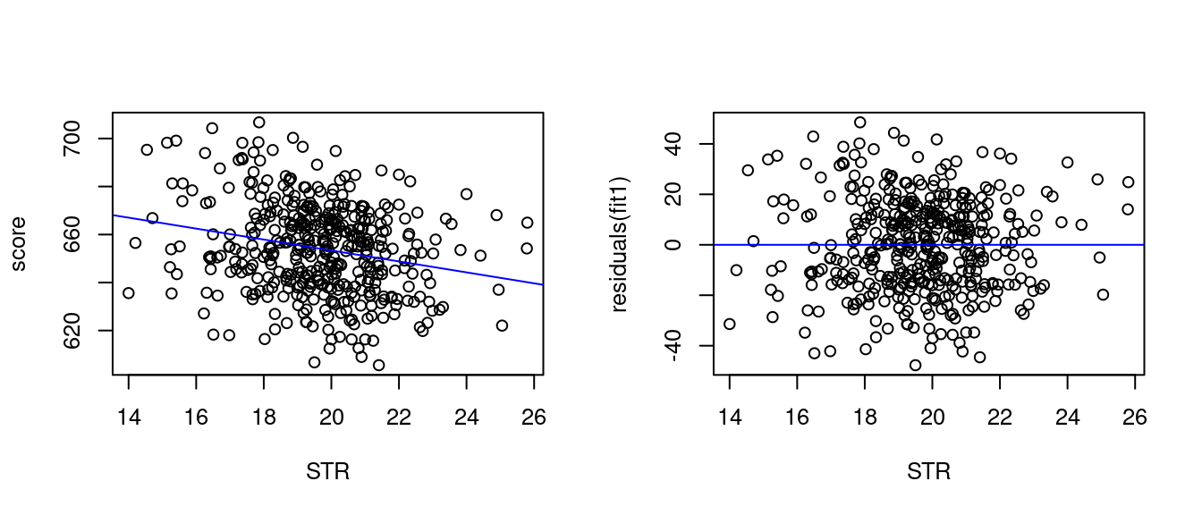
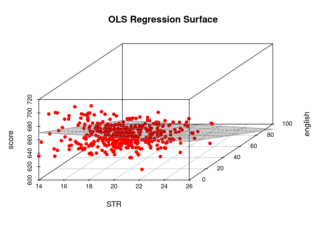
Let’s include the percentage of english learners as an additional regressor:
english = CASchools$english
fit2= lm(score ~ STR + english)
fit2$coefficients
(Intercept) STR english
686.0322445 -1.1012956 -0.6497768 A 3D plot provides a visual representation of the resulting regression line (surface):
Adding the additional predictor income gives a regression specification with dimensions beyond visual representation:
income = CASchools$income
fit3 = lm(score ~ STR + english + income)
fit3$coefficients
(Intercept) STR english income
640.31549821 -0.06877542 -0.48826683 1.49451661 The fitted regression line now includes three predictors and four coefficients: 640.3 - 0.07 \ \text{STR} - 0.49 \ \text{english} + 1.49 \ \text{income}
For specifications with multiple regressors, fitted values and residuals can still be visualized:
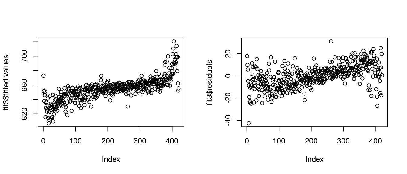
The pattern of fitted values arises because the observations in the CASchools dataset are sorted in ascending order by test score.
3.5 Matrix notation
Matrix notation is convenient because it eliminates the need for summation symbols and indices. We define the response vector \boldsymbol Y and the regressor matrix (design matrix) \boldsymbol X as follows: \boldsymbol Y = \begin{pmatrix} Y_1 \\ Y_2 \\ \vdots \\ Y_n \end{pmatrix}, \quad \boldsymbol X = \begin{pmatrix} \boldsymbol X_1' \\ \boldsymbol X_2' \\ \vdots \\ \boldsymbol X_n' \end{pmatrix} = \begin{pmatrix} 1 & X_{12} & \ldots & X_{1k} \\ \vdots & & & \vdots \\ 1 & X_{n2} &\ldots & X_{nk} \end{pmatrix} Note that \sum_{i=1}^n \boldsymbol X_i \boldsymbol X_i' = \boldsymbol X'\boldsymbol X and \sum_{i=1}^n \boldsymbol X_i Y_i = \boldsymbol X' \boldsymbol Y.
The least squares coefficient vector becomes \widehat{\boldsymbol \beta} = \Big( \sum_{i=1}^n \boldsymbol X_i \boldsymbol X_i' \Big)^{-1} \sum_{i=1}^n \boldsymbol X_i Y_i = (\boldsymbol X'\boldsymbol X)^{-1} \boldsymbol X'\boldsymbol Y. The vector of fitted values can be computed as follows: \widehat{\boldsymbol Y} = \begin{pmatrix} \widehat Y_1 \\ \vdots \\ \widehat Y_n \end{pmatrix} = \boldsymbol X \widehat{\boldsymbol \beta} = \underbrace{\boldsymbol X (\boldsymbol X'\boldsymbol X)^{-1} \boldsymbol X'}_{=\boldsymbol P}\boldsymbol Y = \boldsymbol P \boldsymbol Y. The projection matrix \boldsymbol P is also known as the influence matrix or hat matrix and maps observed values to fitted values.
The vector of residuals is given by \widehat{\boldsymbol u} = \begin{pmatrix} \widehat u_1 \\ \vdots \\ \widehat u_n \end{pmatrix} = \boldsymbol Y - \widehat{\boldsymbol Y} = (\boldsymbol I_n - \boldsymbol P) \boldsymbol Y.
The diagonal entries of \boldsymbol P, given by h_{ii} = \boldsymbol X_i'(\boldsymbol X' \boldsymbol X)^{-1} \boldsymbol X_i, are called leverage values or hat values and measure how far away the regressor values of the i-th observation X_i are from those of the other observations.
Properties of leverage values: 0 \leq h_{ii} \leq 1, \quad \sum_{i=1}^n h_{ii} = k.
A large h_{ii} occurs when the observation i has a big influence on the regression line, e.g., the last observation in the following dataset:
X=c(10,20,30,40,50,60,70,500)
Y=c(1000,2200,2300,4200,4900,5500,7500,10000)
plot(X,Y, main="OLS regression line with and without last observation")
abline(lm(Y~X), col="blue")
abline(lm(Y[1:7]~X[1:7]), col="red")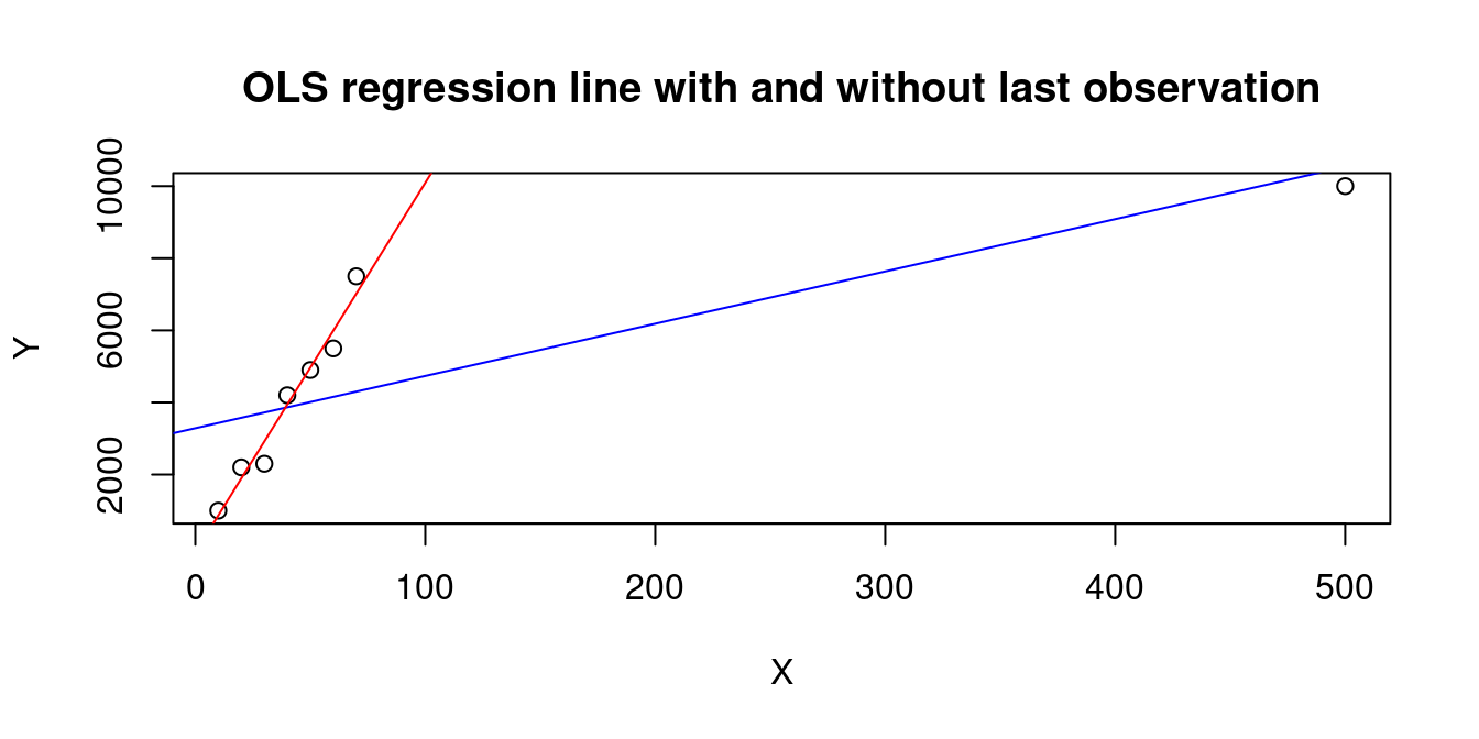
        1         2         3         4         5         6         7         8
0.1657356 0.1569566 0.1492418 0.1425911 0.1370045 0.1324820 0.1290237 0.9869646
3.6 R-squared
Consider the following sample variances:
| Dependent variable | \widehat \sigma_Y^2 = \frac{1}{n} \sum_{i=1}^n (Y_i - \overline Y)^2 |
| Fitted values | \widehat \sigma_{\widehat Y}^2 = \frac{1}{n} \sum_{i=1}^n (\widehat Y_i - \overline{\widehat Y})^2 |
| Residuals | \widehat \sigma_{\widehat u}^2 = \frac{1}{n} \sum_{i=1}^n \widehat u_i^2 |
An important property of the residual vector is that it is orthogonal to the columns of \boldsymbol X, i.e. \boldsymbol X' \widehat{\boldsymbol u} = \begin{pmatrix} \sum_{i=1}^n \widehat u_i \\ \sum_{i=1}^n X_{i2} \widehat u_i \\ \vdots \\ \sum_{i=1}^n X_{ik} \widehat u_i \end{pmatrix} = \begin{pmatrix} 0 \\ 0 \\ \vdots \\ 0 \end{pmatrix}. \tag{3.2} In particular, the sample mean of the residuals is zero, which is why it does not appear in the residual sample variance \widehat \sigma_{\widehat u}^2.
Moreover, the following relationship holds (analysis of variance formula): \widehat \sigma_Y^2 = \widehat \sigma_{\widehat Y}^2 + \widehat \sigma_{\widehat u}^2. Hence, the larger the proportion of the explained sample variance, the better the fit of the OLS regression. This motivates the definition of the R-squared coefficient: R^2 = 1 - \frac{\widehat \sigma_{\widehat u}^2}{\widehat \sigma_{Y}^2} = 1 - \frac{\sum_{i=1}^n \widehat u_i^2}{\sum_{i=1}^n (Y_i - \overline Y)^2} = \frac{\sum_{i=1}^n (\widehat Y_i - \overline{\widehat Y})^2}{\sum_{i=1}^n (Y_i - \overline Y)^2}.
The R-squared describes the proportion of sample variation in \boldsymbol Y explained by \widehat{\boldsymbol Y}. We have 0\leq R^2\leq 1.
In a regression of Y_i on a single regressor Z_i with intercept (simple linear regression), the R-squared is equal to the squared sample correlation coefficient of Y_i and Z_i.
An R-squared of 0 indicates no sample variation in \widehat{\boldsymbol{Y}} (a flat regression line/surface), whereas a value of 1 indicates no variation in \widehat{\boldsymbol{u}}, indicating a perfect fit. The higher the R-squared, the better the OLS regression fits the data.
However, a low R-squared does not necessarily mean the regression specification is bad. It just implies that there is a high share of unobserved heterogeneity in \boldsymbol Y that is not captured by the regressors \boldsymbol X linearly.
Conversely, a high R-squared does not necessarily mean a good regression specification. It just means that the regression fits the sample well. Too many unnecessary regressors lead to overfitting.
If k=n, we have R^2 = 1 even if none of the regressors has an actual influence on the dependent variable.
3.7 Adjusted R-squared
Recall that the deviations (Y_i - \overline Y) cannot vary freely because they are subject to the constraint \sum_{i=1}^n (Y_i - \overline Y), which is why we loose 1 degree of freedom in the sample variance of \boldsymbol Y.
For the sample variance of \widehat{\boldsymbol u}, we loose k degrees of freedom because the residuals are subject to the constraints from Equation 3.2. The adjusted sample variance of the residuals is therefore defined as: s_{\widehat u}^2 = \frac{1}{n-k}\sum_{i=1}^n \widehat u_i^2. By incorporating adjusted versions in the R-squared definition, we penalize regression specifications with large k. The adjusted R-squared is \overline{R}^2 = 1 - \frac{\frac{1}{n-k}\sum_{i=1}^n \widehat u_i^2}{\frac{1}{n-1}\sum_{i=1}^n (Y_i - \overline Y)^2} = 1 - \frac{s_{\widehat u}^2}{s_Y^2}.
The squareroot of the adjusted sample variance of the residuals is called the standard error of the regression (SER) or residual standard error: SER := s_{\widehat u} = \sqrt{ \frac{1}{n-k}\sum_{i=1}^n \widehat u_i^2 }.
The R-squared should be used for interpreting the share of variation explained by the fitted regression line. The adjusted R-squared should be used for comparing different OLS regression specifications.
The commands summary(fit)$r.squared and summary(fit)$adj.r.squared return the R-squared and adjusted R-squared values, respectively. The SER can be returned by summary(fit)$sigma.
The stargazer() function can be used to produce nice regression outputs:
library(stargazer)stargazer(fit1, fit2, fit3, type="html", report="vc*",
omit.stat = "f", star.cutoffs = NA, df=FALSE,
omit.table.layout = "n", digits = 4)| Dependent variable: | |||
| score | |||
| (1) | (2) | (3) | |
| STR | -2.2798 | -1.1013 | -0.0688 |
| english | -0.6498 | -0.4883 | |
| income | 1.4945 | ||
| Constant | 698.9329 | 686.0322 | 640.3155 |
| Observations | 420 | 420 | 420 |
| R2 | 0.0512 | 0.4264 | 0.7072 |
| Adjusted R2 | 0.0490 | 0.4237 | 0.7051 |
| Residual Std. Error | 18.5810 | 14.4645 | 10.3474 |
3.8 Too many regressors
OLS should be considered for regression problems with k << n (small k and large n). When the number of predictors k approaches or equals the number of observations n, we run into the problem of overfitting. Specifically, at k = n, the regression line will perfectly fit the data.
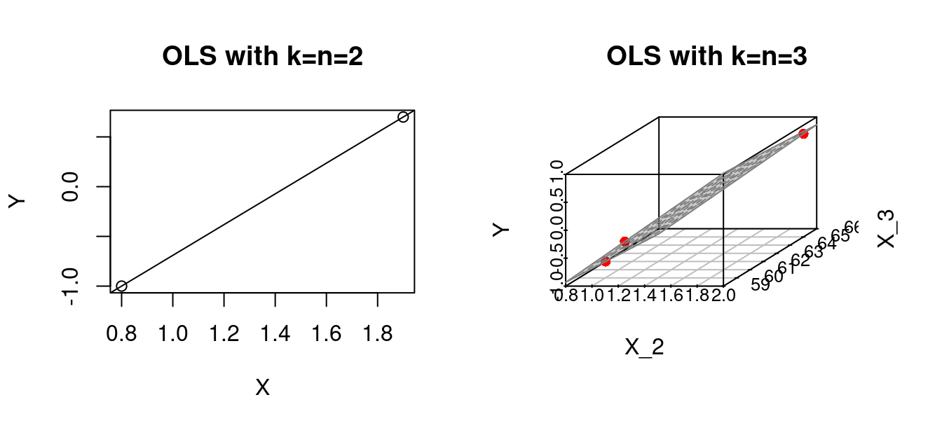
If k=n \geq 4, we can no longer visualize the OLS regression line, but the problem of a perfect fit is still present. If k > n, there exists no OLS solution because \boldsymbol X' \boldsymbol X is not invertible. Regression problems with k \approx n or k>n are called high-dimensional regressions.
3.9 Perfect multicollinearity
The only requirement for computing the OLS coefficients is the invertibility of the matrix \boldsymbol X' \boldsymbol X. As discussed above, a necessary condition is that k \leq n.
Another reason the matrix may not be invertible is if two or more regressors are perfectly collinear. Two variables are perfectly collinear if their sample correlation is 1 or -1. Multicollinearity arises if one variable is a linear combination of the other variables.
Common causes are duplicating a regressor or using the same variable in different units (e.g., GDP in both EUR and USD).
Perfect multicollinearity (or strict multicollinearity) arises if the regressor matrix does not have full column rank: \text{rank}(\boldsymbol X) < k. It implies \text{rank}(\boldsymbol X' \boldsymbol X) < k, so that the matrix is singular and \widehat{\boldsymbol \beta} cannot be computed.
Near multicollinearity occurs when two columns of \boldsymbol X have a sample correlation very close to 1 or -1. Then, (\boldsymbol X' \boldsymbol X) is “near singular”, its eigenvalues are very small, and (\boldsymbol X' \boldsymbol X)^{-1} becomes very large, causing numerical problems.
Multicollinearity means that at least one regressor is redundant and can be dropped.
3.10 Dummy variable trap
A common cause of strict multicollinearity is the inclusion of too many dummy variables. Let’s consider the cps data and add a dummy variable for non-married individuals:
cps = read.csv("cps.csv")
cps$nonmarried = 1-cps$married
fit4 = lm(wage ~ married + nonmarried, data = cps)
fit4$coefficients
(Intercept) married nonmarried
19.338695 6.997155 NA The coefficient for nonmarried is NA. We fell into the dummy variable trap!
The dummy variables married and nonmarried are collinear with the intercept variable because married + nonmarried = 1, which leads to a singular matrix \boldsymbol X' \boldsymbol X.
The solution is to use one dummy variable less than factor levels, as R automatically does by omitting the last dummy variable. Another solution would be to remove the intercept from the model, which can be done by adding -1 to the model formula:
fit5 = lm(wage ~ married + nonmarried - 1, data = cps)
fit5$coefficients
married nonmarried
26.33585 19.33869