A statistical hypothesis is a statement about the population distribution. For instance, we might be interested in the hypothesis that a population regression coefficient \beta_j of a linear regression model is equal to some value \beta_j^0 or whether it is unequal to that value.
For instance, in a regression of test scores on the student-teacher ratio, we might be interested in testing whether adding one more student per class has no effect on test scores – that is, whether \beta_j = \beta_j^0 = 0.
In hypothesis testing, we divide the parameter space of interest into a null hypothesis and an alternative hypothesis, for instance
\underbrace{H_0:\beta_j = \beta_j^0}_{ \text{null hypothesis} } \quad \text{vs.} \quad \underbrace{H_1:\beta_j \neq \beta_j^0.}_{ \text{alternative hypothesis} }
\tag{11.1}
This idea is not limited to regression coefficients. For any parameter \theta we can test the hypothesis H_0: \theta = \theta_0 against its alternative H_1: \theta \neq \theta_0.
In practice, two-sided alternatives are more common, i.e. H_1: \theta \neq \theta_0, but one-sided alternatives are also possible, i.e. H_1: \theta > \theta_0 (right-sided) or H_1: \theta < \theta_0 (left-sided).
We are interested in testing H_0 against H_1. The idea of hypothesis testing is to construct a statistic T_0 (test statistic) for which the distribution of T_0 under the assumption that H_0 holds(null distribution) is known, and for which the distribution under H_1 differs from the null distribution (i.e., the null distribution is informative about H_1).
If the observed value of T_0 takes a value that is likely to occur under the null distribution, we deduce that there is no evidence against H_0, and consequently we do not reject H_0 (we accept H_0). If the observed value of T_0 takes a value that is unlikely to occur under the null distribution, we deduce that there is evidence against H_0, and consequently, we reject H_0 in favor of H_1.
“Unlikely” means that its occurrence has only a small probability \alpha. The value \alpha is called the significance level and must be selected by the researcher. It is conventional to use the values \alpha = 0.1, \alpha=0.05, or \alpha = 0.01, but it is not a hard rule.
A hypothesis test with significance level \alpha is a decision rule defined by a rejection region I_1 and an acceptance region I_0 = I_1^c so that we \begin{align*}
\text{do not reject} \ H_0 \quad \text{if} \ &T_0 \in I_0, \\
\text{reject} \ H_0 \quad \text{if} \ &T_0 \in I_1.
\end{align*} The rejection region is defined such that a false rejection occurs with probability \alpha, i.e.
P( \underbrace{T_0 \in I_1}_{\text{reject}} \mid H_0 \ \text{is true}) = \alpha,
\tag{11.2} where P(\cdot \mid H_0 \ \text{is true}) denotes the probability function of the null distribution.
A test that satisfies Equation 11.2 is called a size-\alpha-test. The type I error is the probability of falsely rejecting H_0 and equals \alpha for a size-\alpha-test. The type II error is the probability of falsely accepting H_0 and depends on the sample size n and the unknown parameter value \theta under H_1. Typically, the further \theta is from \theta_0, and the larger the sample size n, the smaller the type II error.
The probability of a type I error is also called the size of a test:
P( \text{reject} \ H_0 \mid H_0 \ \text{is true}).
The power of a test is the complementary probability of a type II error:
P( \text{reject} \ H_0 \mid H_1 \ \text{is true}) = 1 - P( \text{accept} \ H_0 \mid H_1 \ \text{is true}).
A hypothesis test is consistent for H_1 if the power tends to 1 as n tends to infinity for any parameter value under the alternative.
Testing Decisions
Accept H_0
Reject H_0
H_0 is true
correct decision
type I error
H_1 is true
type II error
correct decision
In many cases, the probability distribution of T_0 under H_0 is known only asymptotically. Then, the rejection region must be defined such that
\lim_{n \to \infty} P( T_0 \in I_1 \mid H_0 \ \text{is true}) = \alpha.
We call this test an asymptotic size-\alpha-test.
The decision “accept H_0” does not mean that H_0 is true. Since the probability of a type II error is unknown in practice, it is more accurate to say that we “fail to reject H_0” instead of “accept H_0”. The power of a consistent test tends to 1 as n increases, so type II errors typically occur if the sample size is too small. Therefore, to interpret a “fail to reject H_0”, we have to consider whether our sample size is relatively small or rather large.
11.2 t-Tests
The t-statistic is the OLS estimator standardized with the standard error. Under (A1)–(A4) we have
T = \frac{\widehat \beta_j - \beta_j}{se_{hc}(\widehat \beta_j)} \overset{d}{\to} \mathcal N(0,1).
This result can be used to test the hypothesis H_0: \beta_j = \beta_j^0. The t-statistic for this hypothesis is
T_0 = \frac{\widehat \beta_j - \beta_j^0}{se_{hc}(\widehat \beta_j)},
which satisfies T_0 = T \overset{d}{\to} \mathcal N(0,1) under H_0.
Therefore, we can test H_0 by checking whether the presumed value \beta_j^0 falls into the confidence interval. We do not reject H_0 if
\beta_j^0 \in I_{1-\alpha}^{(hc)} = \big[\widehat \beta_j - t_{(1-\frac{\alpha}{2},n-k)} se_{hc}(\widehat \beta_j); \ \widehat \beta_j + t_{(1-\frac{\alpha}{2},n-k)} se_{hc}(\widehat \beta_j)\big].
By the definition of T_0, we have \beta_j^0 \in I_{1-\alpha}^{(hc)} if and only if |T_0| \leq t_{(1-\frac{\alpha}{2},n-k)}.
Therefore, the two-sided t-test for H_0 against H_1: \beta_j \neq \beta_j^0 is given by the test decision \begin{align*}
\text{do not reject} \ H_0 \quad \text{if} \ &|T_0| \leq t_{(1-\frac{\alpha}{2},n-k)}, \\
\text{reject} \ H_0 \quad \text{if} \ &|T_0| > t_{(1-\frac{\alpha}{2},n-k)}.
\end{align*}
The value t_{(1-\frac{\alpha}{2},n-k)} is called the critical value.
This test is asymptotically of size \alpha:
\lim_{n \to \infty} P(\text{we reject } H_0| H_0 \text{ is true}) = \alpha.
This is because the confidence interval has asymptotically a 1-\alpha coverage rate: \begin{align*}
&\lim_{n \to \infty} P(\text{we do not reject } H_0| H_0 \text{ is true}) \\
&= \lim_{n \to \infty} P(\beta_j^0 \in I_{1-\alpha}^{(hc)}| H_0 \text{ is true} ) \\
&= \lim_{n \to \infty} P(\beta_j \in I_{1-\alpha}^{(hc)}) \\
&= 1-\alpha.
\end{align*}
If (A5)–(A6) hold, and se_{hom}(\widehat \beta_j) is used instead of se_{hc}(\widehat \beta_j), then the t-test is of exact size \alpha. However, as discussed in the previous section, (A5)–(A6) is an unlikely scenario in practice. Therefore se_{hc}(\widehat \beta_j) is the preferred choice.
library(AER)cps=read.csv("cps.csv")fit=lm(wage~education+female, data =cps)coefci(fit, vcov =vcovHC, level =0.99)
the null hypothesis H_0: \beta_2 = 0 (“the marginal effect of education on the wage conditional on gender is 0”) is rejected at the 1% significance level.
the null hypothesis H_0: \beta_2 = 3 (“the marginal effect of education on the wage conditional on gender is 3”) is not rejected at the 1% significance level.
Let’s compute T_0 for the hypothesis \beta_2 = 3 by hand:
## OLS coefficientbetahat2=fit$coefficient[2]## HC standard errorse=sqrt(vcovHC(fit)[2,2])## presumed value for beta2beta20=3c(betahat2, beta20, se)
 education
2.95817398 3.00000000 0.04011445
## test statisticT0=(betahat2-beta20)/seT0
education
-1.042667
## critical values for 1=%, 5% and 1% levelsn=length(fit$fitted.values)qt(c(0.95, 0.975, 0.995), df=n-3)
[1] 1.644884 1.960011 2.575926
Since |T_0| = 1.04 is smaller that the critical values for all common significance levels, we cannot reject H_0: \beta_2 = 3.
11.3 The p-value
The p-value is a criterion to reach a hypothesis test decision conveniently: \begin{align*}
\text{reject} \ H_0 \quad &\text{if p-value} < \alpha \\
\text{do not reject} \ H_0 \quad &\text{if p-value} \geq \alpha
\end{align*}
Formally, the p-value of a two-sided t-test is defined as
p\text{-value} = P( |T^*| > |T_0| \mid H_0 \ \text{is true}),
where T^* is a random variable following the null distribution (in this case, T^*\sim t_{n-k}), and T_0 is the observed value of the test statistic.
The p-value is the probability that a null-distributed random variable produces values at least as extreme as the test statistic T_0 produced for your sample.
We can express the p-value also using the CDF F_{T_0} of the null distribution (in this case, t_{n-k}): \begin{align*}
p\text{-value} &= P(| T^*| > |T_0| \mid H_0 \ \text{is true}) \\
&= 1 - P(|T^*| \leq |T_0| \mid H_0 \ \text{is true}) \\
&= 1 - F_{T_0}(|T_0|) + F_{T_0}(-|T_0|) \\
&= 2(1 - F_{T_0}(|T_0|)).
\end{align*}
Make no mistake, the p-value is not the probability that H_0 is true! It is a measure of how likely it is that the observed test statistic comes from a sample that has been drawn from a population where the null hypothesis is true.
Let’s compute the p-value for the hypothesis \beta_2 = 3 in the wage on education and female regression by hand. Here, F_{T_0} is the CDF of the t-distribution with n-3 degrees of freedom. To compute F_{T_0}(a), we can use pt(a, df=n-3).
More conveniently, the coeftest function from the AER package provides a full summary of the regression results including the t-statistics and p-values for the hypotheses that H_0:\beta_j=0 for j=1, \ldots, k.
t test of coefficients:

              Estimate Std. Error t value  Pr(>|t|)
(Intercept) -14.081788   0.500136 -28.156 < 2.2e-16 ***
education     2.958174   0.040114  73.743 < 2.2e-16 ***
female       -7.533067   0.161652 -46.601 < 2.2e-16 ***
---
Signif. codes:  0 '***' 0.001 '**' 0.01 '*' 0.05 '.' 0.1 ' ' 1
You can specify different standard errors: coeftest(fit, vcov = vcovHC, type = "HC1"). coeftest(fit) returns the t-test results for classical standard errors which is identical to the output of the base-R command summary(fit), which should not be used in applications with heteroskedasticity.
To represent very small numbers where there are, e.g., 16 zero digits before the first nonzero digit after the decimal point, R uses scientific notation in the form e-16. For example, 2.2e-16 means 0.00000000000000022.
11.4 Multiple testing problem
Consider the usual two-sided t-tests for the hypotheses H_0: \beta_1 = 0 (test1) and H_0: \beta_2 = 0 (test2).
Each test on its own is a valid hypothesis test of size \alpha. However, applying these tests one after the other leads to a multiple testing problem. The probability of falsely rejecting the joint hypothesis
H_0: \beta_1 = 0 \ \text{and} \ \beta_2 = 0 \quad \text{vs.} \quad H_1: \text{not} \ H_0
is too large. “Not H_0” means “\beta_1 \neq 0 \ \text{or} \ \beta_2 \neq 0 \ \text{or both}”.
To see this, suppose that, for simplicity, the t-statistics \widehat \beta_1/se(\widehat \beta_1) and \widehat \beta_2/se(\widehat \beta_2) are independent random variables, which implies that the test decisions of the two tests are independent. \begin{align*}
&P(\text{both tests do not reject} \mid H_0 \ \text{true}) \\
&=P(\{\text{test1 does not reject}\} \cap \{\text{test2 does not reject}\} \mid H_0 \ \text{true}) \\
&= P(\text{test1 does not reject} \mid H_0 \ \text{true}) \cdot P(\text{test2 does not reject} \mid H_0 \ \text{true}) \\
&= (1-\alpha)^2 = \alpha^2 - 2\alpha + 1
\end{align*}
The size of the combined test is larger than \alpha: \begin{align*}
&P(\text{at least one test rejects} \mid H_0 \ \text{is true}) \\
&= 1 - P(\text{both tests do not reject} \mid H_0 \ \text{is true}) \\
&= 1 - (\alpha^2 - 2\alpha + 1) = 2\alpha - \alpha^2 = \alpha(2-\alpha) > \alpha
\end{align*}
If the two test statistics are dependent, then the probability of at least one of the tests falsely rejecting depends on their correlation and will also exceed \alpha.
Each t-test has a probability of falsely rejecting H_0 (type I error) of \alpha, but if multiple t-tests are used on different coefficients, then the probability of falsely rejecting at least once (joint type I error probability) is greater than \alpha (multiple testing problem).
Therefore, when multiple hypotheses are to be tested, repeated t-tests will not yield valid inferences, and another rejection rule must be found for repeated t-tests.
11.5 Joint Hypotheses
Consider the general hypothesis
H_0: \boldsymbol R \boldsymbol \beta = \boldsymbol r,
where \boldsymbol R is a q \times k matrix with \text{rank}(\boldsymbol R) = q and \boldsymbol r is a q \times 1 vector.
Let’s look at a linear regression with k=3: \begin{align*}
Y_i = \beta_1 + \beta_2 X_{i2} + \beta_3 X_{i3} + u_i
\end{align*}
Example 1: The hypothesis H_0 : (\beta_2 = 0 and \beta_3 = 0) implies q=2 constraints and is translated to H_0: \boldsymbol R \boldsymbol \beta = \boldsymbol r with
\boldsymbol R = \begin{pmatrix}
0 & 1 & 0 \\
0 & 0 & 1
\end{pmatrix} , \quad \boldsymbol r = \begin{pmatrix}
0 \\ 0
\end{pmatrix}.
Example 2: The hypothesis H_0: \beta_2 + \beta_3 = 1 implies q=1 constraint and is translated to H_0: \boldsymbol R \boldsymbol \beta = \boldsymbol r with
\boldsymbol R = \begin{pmatrix}
0 & 1 & 1
\end{pmatrix} , \quad \boldsymbol r = \begin{pmatrix}
1
\end{pmatrix}.
In practice, the most common multiple hypothesis tests are tests of whether multiple coefficients are equal to zero, which is a test of whether those regressors should be included in the model.
11.6 Wald Test
The Wald distance is the vector \boldsymbol d = \boldsymbol R\widehat{\boldsymbol \beta} - \boldsymbol r, and the Wald statistic is the squared standardized Wald distance vector: \begin{align*}
W &= \boldsymbol d' (\boldsymbol R \widehat{\boldsymbol V} \boldsymbol R')^{-1} \boldsymbol d \\
&= (\boldsymbol R\widehat{\boldsymbol \beta} - \boldsymbol r)'(\boldsymbol R \widehat{\boldsymbol V} \boldsymbol R')^{-1} (\boldsymbol R\widehat{\boldsymbol \beta} - \boldsymbol r)
\end{align*} Here, \widehat{\boldsymbol V} is a suitable estimator for covariance matrix of the OLS coefficient vector, i.e. \widehat{\boldsymbol V}_{hc} for robust testing under (A1)–(A4), and \widehat{\boldsymbol V}_{hom} for testing under the special case of homoskedasticity.
Under H_0 we have
W \overset{d}{\to} \chi^2_q.
The test decision for the Wald test: \begin{align*}
\text{do not reject} \ H_0 \quad \text{if} \ &W \leq \chi^2_{(1-\alpha, q)}, \\
\text{reject} \ H_0 \quad \text{if} \ &W > \chi^2_{(1-\alpha,q)},
\end{align*} where \chi^2_{(p,q)} is the p-quantile of the chi-squared distribution with q degrees of freedom. \chi^2_{(p,q)} can be returned using qchisq(p,q).
To test H_0: \beta_2 = \beta_3 = 0 in the regression of wage on education and female (example 1), we can use the linearHypothesis() function from the AER package:
## Define r and Rr=c(0,0)R=rbind(c(0,1,0),c(0,0,1))R
     [,1] [,2] [,3]
[1,]    0    1    0
[2,]    0    0    1
linearHypothesis(fit, hypothesis.matrix =R, rhs =r, vcov =vcovHC, test ="Chisq")
The null hypothesis is rejected because the p-value is very small. To confirm this, we see in the output that the Wald statistic is W = 5977. The critical value for the common significance levels are:
If vcov = vcovHC is omitted, then the homoskedasticity-only covariance matrix \widehat{\boldsymbol V}_{hom} is used. If test = "Chisq is omitted, then the F-test is applied, which is introduced below.
11.7 F-Test
The Wald test is an asymptotic size-\alpha-test under (A1)–(A4). Even if (A5) and (A6) hold true as well, the Wald test is still only asymptotically valid, i.e.:
\lim_{n \to \infty} P( \text{Wald test rejects} \ H_0 | H_0 \ \text{true} ) = \alpha.
Similarly to the classical t-test, we can construct a test joint test that is of exact size \alpha under (A1)–(A6).
The F statistic is the Wald statistic scaled by the number of constraints:
F = \frac{W}{q} = \frac{1}{q} (\boldsymbol R\widehat{\boldsymbol \beta} - \boldsymbol r)'(\boldsymbol R \widehat{\boldsymbol V} \boldsymbol R')^{-1} (\boldsymbol R\widehat{\boldsymbol \beta} - \boldsymbol r).
If (A1)–(A6) hold true, and if \widehat{\boldsymbol V} = \widehat{\boldsymbol V}_{hom} is used, it can be shown that
F \sim F_{q;n-k}
for any finite sample size n, where F_{q;n-k} is the F-distribution with q degrees of freedom in the numerator and n-k degrees of freedom in the denominator.
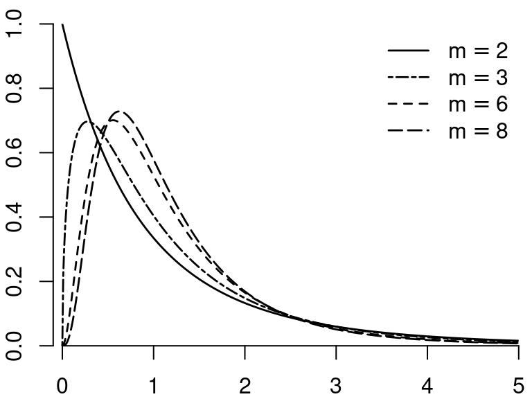
F-distribution
If Q_1 \sim \chi^2_m and Q_2 \sim \chi^2_r, and if Q_1 and Q_2 are independent, then
Y = \frac{Q_1/m}{Q_2/r}
is F-distributed with parameters m and r, written Y \sim F_{m,r}.
The parameter m is called the degrees of freedom in the numerator; r is the degree of freedom in the denominator.
If r \to \infty then the distribution of mY approaches \chi^2_m
Figure 11.1: F-distribution
F-test decision rule
The test decision for the F-test: \begin{align*}
\text{do not reject} \ H_0 \quad \text{if} \ &F \leq F_{(1-\alpha,q,n-k)}, \\
\text{reject} \ H_0 \quad \text{if} \ &F > F_{(1-\alpha,q,n-k)},
\end{align*} where F_{(p,m_1,m_2)} is the p-quantile of the F distribution with m_1 degrees of freedom in the numerator and m_2 degrees of freedom in the denominator. F_{(p,m_1,m_2)} can be returned using qf(p,m1,m2).
For single constraint (q=1) hypotheses of the form H_0: \beta_j = \beta_j^0, the F-test is equivalent to a two-sided t-test.
If (A1)–(A6) hold true and \widehat{\boldsymbol V} = \widehat{\boldsymbol V}_{hom} is used, the F-test has exact size \alpha, similar to the exact t-test for this case.
If (A1)–(A5) hold true and \widehat{\boldsymbol V} = \widehat{\boldsymbol V}_{hom} is used, the F-test and the Wald-test have asymptotic size \alpha.
If (A1)–(A4) hold true and \widehat{\boldsymbol V} = \widehat{\boldsymbol V}_{hc} is used, the F-test and the Wald-test have asymptotic size \alpha.
The F-test tends to be more conservative than the Wald test in small samples, meaning that rejection by the F-test generally implies rejection by the Wald test, but not necessarily vice versa. Due to this more conservative nature, which helps control false rejections (Type I errors) in small samples, the F-test is often preferred in practice.
Linear hypothesis test

Hypothesis:
education = 0
female = 0

Model 1: restricted model
Model 2: wage ~ education + female

Note: Coefficient covariance matrix supplied.

  Res.Df Df      F    Pr(>F)
1  50741
2  50739  2 2988.7 < 2.2e-16 ***
---
Signif. codes:  0 '***' 0.001 '**' 0.01 '*' 0.05 '.' 0.1 ' ' 1
Here, we have F = W/2. The critical values for the common significance level can be obtained as follows:
n=length(fit$fitted.values)k=3q=2qf(c(0.9, 0.95, 0.99), q, n-k)
[1] 2.302690 2.995909 4.605588
Since F = 2988.7, the null hypothesis is rejected at all common significance levels.
11.8 Diagnostics tests
The asymptotic properties of the OLS estimator and inferential methods using HC-type standard errors do not depend on the validity of the homoskedasticity and normality assumptions (A5)–(A6).
However, if you are interested in exact inference, verifying the assumptions (A5)–(A6) becomes crucial, especially in small samples.
11.8.1 Breusch-Pagan Test (Koenker’s version)
Under homoskedasticity, the variance of the error term does not depend on the values of the regressors.
To test for heteroskedasticity, we regress the squared residuals on the regressors.
\widehat u_i^2 = \boldsymbol X_i' \boldsymbol \gamma + v_i, \quad i=1, \ldots, n.
\tag{11.3} Here, \boldsymbol \gamma are the auxiliary coefficients and v_i are the auxiliary error terms. Under homoskedasticity, the regressors should not be able to explain any variation in the residuals.
Let R^2_{aux} be the R-squared coefficient of the auxiliary regression of Equation 11.3. The test statistic:
BP = n R^2_{aux}
Under the null hypothesis of homoskedasticity, we have
BP \overset{d}{\to} \chi^2_{k-1}
Test decision rule: Reject H_0 if BP exceeds \chi^2_{(1-\alpha,k-1)}.
In R we can apply the bptest() function from the AER package to the lm object of our regression.
    studentized Breusch-Pagan test

data:  fit
BP = 1070.3, df = 2, p-value < 2.2e-16
The BP test clearly rejects H_0, which is strong statistical evidence that the errors are heteroskedastic.
11.8.2 Jarque-Bera Test
A general property of any normally distributed random variable is that it has a skewness of 0 and a kurtosis of 3.
Under (A5)–(A6), we have u_i \sim \mathcal N(0,\sigma^2), which implies E[u_i^3] = 0 and E[u_i^4] = 3 \sigma^4.
Consider the sample skewness and the sample kurtosis of the residuals from your regression:
\widehat{skew}_{\widehat u} = \frac{1}{n \widehat \sigma_{\widehat u}^3} \sum_{i=1}^n \widehat u_i^3, \quad
\widehat{kurt}_{\widehat u} = \frac{1}{n \widehat \sigma_{\widehat u}^4} \sum_{i=1}^n \widehat u_i^4
Jarque-Bera test statistic and null distribution if (A5)–(A6) hold:
JB = n \bigg( \frac{1}{6} \big(\widehat{skew}_{\widehat u}\big)^2 + \frac{1}{24} \big(\widehat{kurt}_{\widehat u} - 3\big)^2 \bigg) \overset{d}{\to} \chi^2_2.
Test decision rule: Reject the null hypothesis of normality if JB exceeds \chi^2_{(1-\alpha,2)}.
Note that the Jarque-Bera test is sensitive to outliers.
In R we apply use the jarque.test() function from the moments package to the residual vector from our regression.
    Jarque-Bera Normality Test

data:  fit$residuals
JB = 2230900, p-value < 2.2e-16
alternative hypothesis: greater
The JB test clearly rejects H_0, which is strong statistical evidence that the errors are not normally distributed.
The results of the BP and the JB test indicate that classical standard errors se(\beta_j) and the classical covariance matrix estimators \widehat{\boldsymbol V}_{hom} should not be used. Instead, HC-versions should be applied.
11.9 Nonliearities in test score regressions
Let’s use the hypothesis tests from this section to conduct a study on the relationship between test scores and the student-teacher ratio.
data(CASchools, package ="AER")## append student-teacher ratioCASchools$STR=CASchools$students/CASchools$teachers## append average test scoreCASchools$score=(CASchools$read+CASchools$math)/2## append high English learner share dummy variableCASchools$HiEL=(CASchools$english>=10)|>as.numeric()
This section examines three key questions about test scores and the student-teacher ratio.
First, it explores if reducing the student-teacher ratio affects test scores differently based on the number of English learners, even when considering economic differences across districts.
Second, it investigates if this effect varies depending on the student-teacher ratio.
Lastly, it aims to determine the expected impact on test scores when the student-teacher ratio decreases by two students per teacher, considering both economic factors and potential nonlinear relationships.
The logarithm of district income is used following our previous empirical analysis, which suggested that this specification captures the nonlinear relationship between scores and income.
We leave out the expenditure per pupil (expenditure) from our analysis because including it would suggest that spending changes with the student-teacher ratio (in other words, we would not be holding expenditures per pupil constant: bad control).
We will consider 7 different model specifications:
# estimate all modelsmod1=lm(score~STR+english+lunch, data =CASchools)mod2=lm(score~STR+english+lunch+log(income), data =CASchools)mod3=lm(score~STR+HiEL+HiEL:STR, data =CASchools)mod4=lm(score~STR+HiEL+HiEL:STR+lunch+log(income), data =CASchools)mod5=lm(score~STR+I(STR^2)+I(STR^3)+HiEL+lunch+log(income), data =CASchools)mod6=lm(score~STR+I(STR^2)+I(STR^3)+HiEL+HiEL:STR+HiEL:I(STR^2)+HiEL:I(STR^3)+lunch+log(income), data =CASchools)mod7=lm(score~STR+I(STR^2)+I(STR^3)+english+lunch+log(income), data =CASchools)# gather robust standard errors in a listrob_se=list(sqrt(diag(vcovHC(mod1))),sqrt(diag(vcovHC(mod2))),sqrt(diag(vcovHC(mod3))),sqrt(diag(vcovHC(mod4))),sqrt(diag(vcovHC(mod5))),sqrt(diag(vcovHC(mod6))),sqrt(diag(vcovHC(mod7))))
The stars in the regression output indicate the statistical significance of each coefficient based on a t-test of the hypothesis H_0: \beta_j = 0. No stars indicate that the coefficient is not statistically significant (cannot reject H_0 at conventional significance levels). One star (^*) denotes significance at the 10% level (pval < 0.10), two stars (^{**}) indicate significance at the 5% level (pval < 0.05), and three stars (^{***}) indicate significance at the 1% level (pval < 0.01).
What can be concluded from the results presented?
First, we find that there is evidence of heteroskedasticity and non-normality, because the Breusch-Pagan test and the Jarque-Bera test reject. Therefore, HC-robust tests should be used.
    Jarque-Bera Normality Test

data:  mod1$residuals
JB = 10.626, p-value = 0.004926
alternative hypothesis: greater
We see the estimated coefficient of STR is highly significant in all models except from specifications (3) and (4).
When we add log(income) to model (1) in the second specification, all coefficients remain highly significant while the coefficient on the new regressor is also statistically significant at the 1% level. In addition, the coefficient on STR is now 0.27 higher than in model (1), which suggests a possible reduction in omitted variable bias when including log(income) as a regressor. For these reasons, it makes sense to keep this variable in other models too.
Models (3) and (4) include the interaction term between STR and HiEL, first without control variables in the third specification and then controlling for economic factors in the fourth. The estimated coefficient for the interaction term is not significant at any common level in any of these models, nor is the coefficient on the dummy variable HiEL. However, this result is misleading and we should not conclude that none of the variables has a non-zero marginal effect because the coefficients cannot be interpreted separately from each other. What we can learn from the fact that the coefficient of STR:HiEL alone is not significantly different from zero is that the impact of the student-teacher ratio on test scores remains consistent across districts with high and low proportions of English learning students. Let’s test the hypotheses that all coefficients that involve STR are zero and all coefficients that involve HiEL are zero. We find that H_0 is rejected for both hypotheses and the overall marginal effects are clearly significant:
Linear hypothesis test

Hypothesis:
HiEL = 0
STR:HiEL = 0

Model 1: restricted model
Model 2: score ~ STR + HiEL + HiEL:STR

Note: Coefficient covariance matrix supplied.

  Res.Df Df      F    Pr(>F)
1    418
2    416  2 88.806 < 2.2e-16 ***
---
Signif. codes:  0 '***' 0.001 '**' 0.01 '*' 0.05 '.' 0.1 ' ' 1
In regression (5) we have included quadratic and cubic terms for STR, while omitting the interaction term between STR and HiEL, since it was not significant in specification (4). The results indicate high levels of significance for these estimated coefficients and we can therefore assume the presence of a nonlinear effect of the student-teacher ration on test scores. This can be verified with an F-test of H_0: \beta_3 = \beta_4 =0:
Regression (6) further examines whether the proportion of English learners influences the student-teacher ratio, incorporating the interaction terms HiEL\cdot STR, HiEL\cdot STR^2 and HiEL\cdot STR^3. Each individual t-test confirms significant effects. To validate this, we perform a robust F-test to assess H_0: \beta_8 = \beta_9 = \beta_10 =0.
With a p-value of 0.08882 we can just reject the null hypothesis at the 10% level. This provides only weak evidence that the regression functions are different for districts with high and low percentages of English learners.
In model (7), we employ a continuous measure for the proportion of English learners instead of a dummy variable (thus omitting interaction terms). We note minimal alterations in the coefficient estimates for the remaining regressors. Consequently, we infer that the findings observed in model (5) are robust and not influenced significantly by the method used to measure the percentage of English learners.
We can now address the initial questions raised in this section:
First, in the linear models, the impact of the percentage of English learners on changes in test scores due to variations in the student-teacher ratio is minimal, a conclusion that holds true even after accounting for students’ economic backgrounds. Although the cubic specification (6) suggests that the relationship between student-teacher ratio and test scores is influenced by the proportion of English learners, the magnitude of this influence is not significant.
Second, while controlling for students’ economic backgrounds, we identify nonlinearities in the association between student-teacher ratio and test scores.
Lastly, under the linear specification (2), a reduction of two students per teacher in the student-teacher ratio is projected to increase test scores by approximately 1.46 points. As this model is linear, this effect remains consistent regardless of class size. For instance, assuming a student-teacher ratio of 20, the nonlinear model (5) indicates that the reduction in student-teacher ratio would lead to an increase in test scores by \begin{align*}
\small
&64.33 \cdot 18 + 18^2 \cdot (-3.42) + 18^3 \cdot (0.059) \\
&\quad - (64.33 \cdot 20 + 20^2 \cdot (-3.42) + 20^3 \cdot (0.059)) \\
&\approx 3.3
\end{align*} points. If the ratio was 22, a reduction to 20 leads to a predicted improvement in test scores of \begin{align*}
\small
&64.33 \cdot 20 + 20^2 \cdot (-3.42) + 20^3 \cdot (0.059) \\
&\quad - (64.33 \cdot 22 + 22^2 \cdot (-3.42) + 22^3 \cdot (0.059)) \\
&\approx 2.4
\end{align*} points. This suggests that the effect is more evident in smaller classes.